The LAB

Chapter 1. Vectors, scalars, and geometry

1. Scalars, Vectors, and Coordinate Systems

Let’s get our hands dirty! This lab is about playing with the building blocks of linear algebra: scalars and vectors. Think of a scalar as just a plain number, like 3 or -1.5. A vector is a small list of numbers, which you can picture as an arrow in space.

We’ll use Python (with NumPy) to explore them. Don’t worry if this is your first time with NumPy – we’ll go slowly.

Set Up Your Lab

import numpy as np

That’s it – we’re ready! NumPy is the main tool we’ll use for linear algebra.

Step-by-Step Code Walkthrough

Scalars are just numbers.

= 5       # a scalar
= -2.5    # another scalar

print(a + b)   # add them
print(a * b)   # multiply them

2.5
-12.5

Vectors are lists of numbers.

= np.array([2, 3])      # a vector in 2D
= np.array([1, -1, 4])  # a vector in 3D

print(v)
print(w)

[2 3]
[ 1 -1  4]

Coordinates tell us where we are. Think of [2, 3] as “go 2 steps in the x-direction, 3 steps in the y-direction.”

We can even draw it:

import matplotlib.pyplot as plt

# plot vector v
0, 0, v[0], v[1], angles='xy', scale_units='xy', scale=1, color='r')
0, 4)
0, 4)

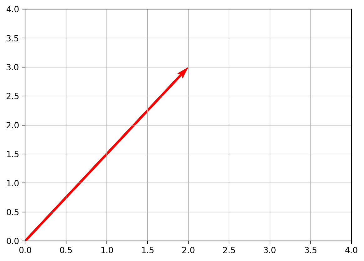
This makes a little arrow from the origin (0,0) to (2,3).

Try It Yourself

Change the vector v to [4, 1]. Where does the arrow point now?
Try making a 3D vector with 4 numbers, like [1, 2, 3, 4]. What happens?
Replace np.array([2,3]) with np.array([0,0]). What does the arrow look like?

2. Vector Notation, Components, and Arrows

In this lab, we’ll practice reading, writing, and visualizing vectors in different ways. A vector can look simple at first – just a list of numbers – but how we write it and how we interpret it really matters. This is where notation and components come into play.

A vector has:

A symbol (we might call it v, w, or even →AB in geometry).
Components (the individual numbers, like 2 and 3 in [2, 3]).
An arrow picture (a geometric way to see the vector as a directed line segment).

Let’s see all three in action with Python.

Set Up Your Lab

import numpy as np
import matplotlib.pyplot as plt

Step-by-Step Code Walkthrough

Writing vectors in Python

# Two-dimensional vector
= np.array([2, 3])

# Three-dimensional vector
= np.array([1, -1, 4])

print("v =", v)
print("w =", w)

v = [2 3]
w = [ 1 -1  4]

Here v has components (2, 3) and w has components (1, -1, 4).

Accessing components Each number in the vector is a component. We can pick them out using indexing.

print("First component of v:", v[0])
print("Second component of v:", v[1])

First component of v: 2
Second component of v: 3

Notice: in Python, indices start at 0, so v[0] is the first component.

Visualizing vectors as arrows In 2D, it’s easy to draw a vector from the origin (0,0) to its endpoint (x,y).

0, 0, v[0], v[1], angles='xy', scale_units='xy', scale=1, color='r')
-1, 4)
-2, 4)
0, color='black', linewidth=0.5)
0, color='black', linewidth=0.5)

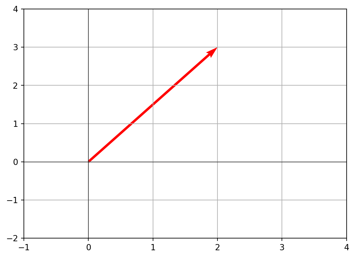
This shows vector v as a red arrow from (0,0) to (2,3).

Drawing multiple vectors We can plot several arrows at once to compare them.

= np.array([3, 1])
= np.array([-1, 2])

# Draw v, u, z in different colors
0, 0, v[0], v[1], angles='xy', scale_units='xy', scale=1, color='r', label='v')
0, 0, u[0], u[1], angles='xy', scale_units='xy', scale=1, color='b', label='u')
0, 0, z[0], z[1], angles='xy', scale_units='xy', scale=1, color='g', label='z')

-2, 4)
-2, 4)
0, color='black', linewidth=0.5)
0, color='black', linewidth=0.5)

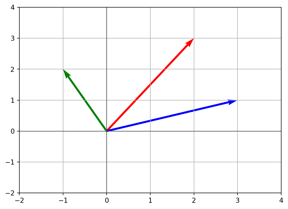
Now you’ll see three arrows starting at the same point, each pointing in a different direction.

Try It Yourself

Change v to [5, 0]. What does the arrow look like now?
Try a vector like [0, -3]. Which axis does it line up with?
Make a new vector q = np.array([2, 0, 0]). What happens if you try to plot it with plt.quiver in 2D?

3. Vector Addition and Scalar Multiplication

In this lab, we’ll explore the two most fundamental operations you can perform with vectors: adding them together and scaling them by a number (a scalar). These operations form the basis of everything else in linear algebra, from geometry to machine learning. Understanding how they work, both in code and visually, is key to building intuition.

Set Up Your Lab

import numpy as np
import matplotlib.pyplot as plt

Step-by-Step Code Walkthrough

Vector addition When you add two vectors, you simply add their components one by one.

= np.array([2, 3])
= np.array([1, -1])

= v + u
print("v + u =", sum_vector)

v + u = [3 2]

Here, (2,3) + (1,-1) = (3,2).

Visualizing vector addition (tip-to-tail method) Graphically, vector addition means placing the tail of one vector at the head of the other. The resulting vector goes from the start of the first to the end of the second.

0, 0, v[0], v[1], angles='xy', scale_units='xy', scale=1, color='r', label='v')
0], v[1], u[0], u[1], angles='xy', scale_units='xy', scale=1, color='b', label='u placed at end of v')
0, 0, sum_vector[0], sum_vector[1], angles='xy', scale_units='xy', scale=1, color='g', label='v + u')

-1, 5)
-2, 5)
0, color='black', linewidth=0.5)
0, color='black', linewidth=0.5)

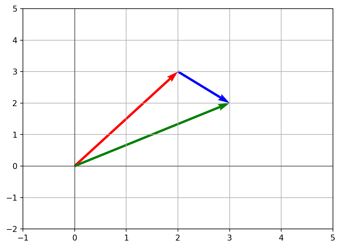
The green arrow is the result of adding v and u.

Scalar multiplication Multiplying a vector by a scalar stretches or shrinks it. If the scalar is negative, the vector flips direction.

= 2
= c * v
print("2 * v =", scaled_v)

= -1
= d * v
print("-1 * v =", scaled_v_neg)

2 * v = [4 6]
-1 * v = [-2 -3]

So 2 * (2,3) = (4,6) and -1 * (2,3) = (-2,-3).

Visualizing scalar multiplication

0, 0, v[0], v[1], angles='xy', scale_units='xy', scale=1, color='r', label='v')
0, 0, scaled_v[0], scaled_v[1], angles='xy', scale_units='xy', scale=1, color='b', label='2 * v')
0, 0, scaled_v_neg[0], scaled_v_neg[1], angles='xy', scale_units='xy', scale=1, color='g', label='-1 * v')

-5, 5)
-5, 7)
0, color='black', linewidth=0.5)
0, color='black', linewidth=0.5)

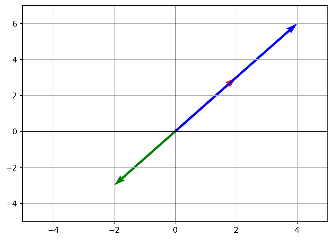
Here, the blue arrow is twice as long as the red arrow, while the green arrow points in the opposite direction.

Combining both operations We can scale vectors and then add them. This is called a linear combination (and it’s the foundation for the next section).

= 3*v + (-2)*u
print("3*v - 2*u =", combo)

3*v - 2*u = [ 4 11]

Try It Yourself

Replace c = 2 with c = 0.5. What happens to the vector?
Try adding three vectors: v + u + np.array([-1,2]). Can you predict the result before printing?
Visualize 3*v + 2*u using arrows. How does it compare to just v + u?

4. Linear Combinations and Span

Now that we know how to add vectors and scale them, we can combine these two moves to create linear combinations. A linear combination is just a recipe: multiply vectors by scalars, then add them together. The set of all possible results you can get from such recipes is called the span.

This idea is powerful because span tells us what directions and regions of space we can reach using given vectors.

Set Up Your Lab

import numpy as np
import matplotlib.pyplot as plt

Step-by-Step Code Walkthrough

Linear combinations in Python

= np.array([2, 1])
= np.array([1, 3])

= 2*v + 3*u
= -1*v + 4*u

print("2*v + 3*u =", combo1)
print("-v + 4*u =", combo2)

2*v + 3*u = [ 7 11]
-v + 4*u = [ 2 11]

Here, we multiplied and added vectors using scalars. Each result is a new vector.

Visualizing linear combinations Let’s plot v, u, and their combinations.

0, 0, v[0], v[1], angles='xy', scale_units='xy', scale=1, color='r', label='v')
0, 0, u[0], u[1], angles='xy', scale_units='xy', scale=1, color='b', label='u')
0, 0, combo1[0], combo1[1], angles='xy', scale_units='xy', scale=1, color='g', label='2v + 3u')
0, 0, combo2[0], combo2[1], angles='xy', scale_units='xy', scale=1, color='m', label='-v + 4u')

-5, 10)
-5, 10)
0, color='black', linewidth=0.5)
0, color='black', linewidth=0.5)

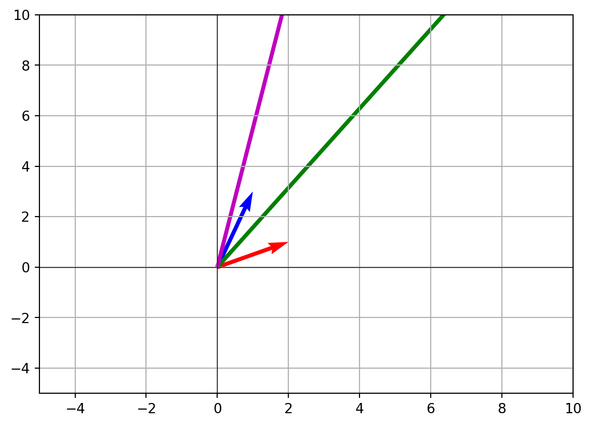
This shows how new arrows can be generated from scaling and adding the original ones.

Exploring the span The span of two 2D vectors is either:

A line (if one is a multiple of the other).
The whole 2D plane (if they are independent).

# Generate many combinations
= range(-5, 6)
= []
for a in coeffs:
for b in coeffs:
= a*v + b*u


= np.array(points)

0], points[:,1], s=10, color='gray')
0, 0, v[0], v[1], angles='xy', scale_units='xy', scale=1, color='r')
0, 0, u[0], u[1], angles='xy', scale_units='xy', scale=1, color='b')

-10, 10)
-10, 10)
0, color='black', linewidth=0.5)
0, color='black', linewidth=0.5)

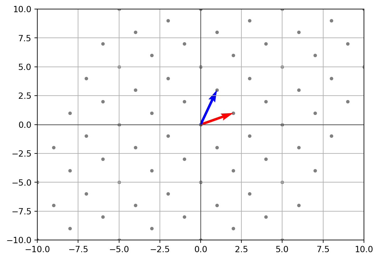
The gray dots show all reachable points with combinations of v and u.

Special case: dependent vectors

= np.array([4, 2])  # notice w = 2*v
= range(-5, 6)
= []
for a in coeffs:
for b in coeffs:
*v + b*w)

= np.array(points)

0], points[:,1], s=10, color='gray')
0, 0, v[0], v[1], angles='xy', scale_units='xy', scale=1, color='r')
0, 0, w[0], w[1], angles='xy', scale_units='xy', scale=1, color='b')

-10, 10)
-10, 10)
0, color='black', linewidth=0.5)
0, color='black', linewidth=0.5)

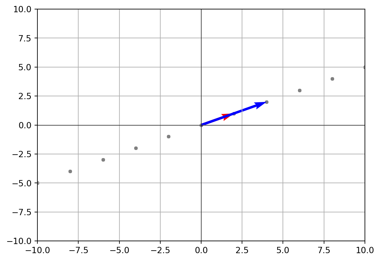
Here, the span collapses to a line because w is just a scaled copy of v.

Try It Yourself

Replace u = [1,3] with u = [-1,2]. What does the span look like?
Try three vectors in 2D (e.g., v, u, w). Do you get more than the whole plane?
Experiment with 3D vectors. Use np.array([x,y,z]) and check whether different vectors span a plane or all of space.

5. Length (Norm) and Distance

In this lab, we’ll measure how big a vector is (its length, also called its norm) and how far apart two vectors are (their distance). These ideas connect algebra to geometry: when we compute a norm, we’re measuring the size of an arrow; when we compute a distance, we’re measuring the gap between two points in space.

Set Up Your Lab

import numpy as np
import matplotlib.pyplot as plt

Step-by-Step Code Walkthrough

Vector length (norm) in 2D The length of a vector is computed using the Pythagorean theorem. For a vector (x, y), the length is sqrt(x² + y²).

= np.array([3, 4])
= np.linalg.norm(v)
print("Length of v =", length)

Length of v = 5.0

This prints 5.0, because (3,4) forms a right triangle with sides 3 and 4, and sqrt(3²+4²)=5.

Manual calculation vs NumPy

= (v[0]**2 + v[1]**2)**0.5
print("Manual length =", manual_length)
print("NumPy length =", np.linalg.norm(v))

Manual length = 5.0
NumPy length = 5.0

Both give the same result.

Visualizing vector length

0, 0, v[0], v[1], angles='xy', scale_units='xy', scale=1, color='r')
0, 5)
0, 5)
0, color='black', linewidth=0.5)
0, color='black', linewidth=0.5)
0]/2, v[1]/2, f"Length={length}", fontsize=10, color='blue')

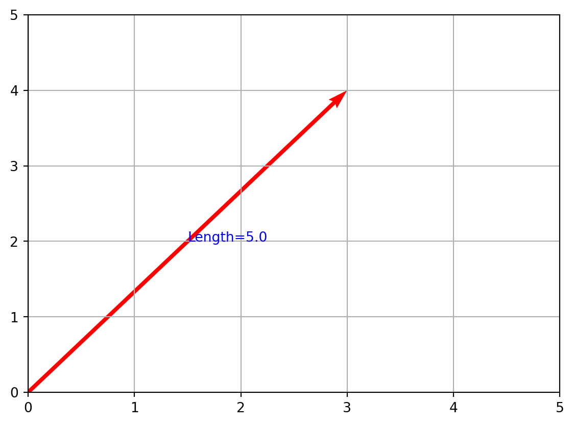
You’ll see the arrow (3,4) with its length labeled.

Distance between two vectors The distance between v and another vector u is the length of their difference: ‖v - u‖.

= np.array([0, 0])   # the origin
= np.linalg.norm(v - u)
print("Distance between v and u =", dist)

Distance between v and u = 5.0

Since u is the origin, this is just the length of v.

A more interesting distance

= np.array([1, 1])
= np.linalg.norm(v - u)
print("Distance between v and u =", dist)

Distance between v and u = 3.605551275463989

This measures how far (3,4) is from (1,1).

Visualizing distance between points

0], u[0]], [v[1], u[1]], color=['red','blue'])
0], u[0]], [v[1], u[1]], 'k--')
0], v[1], 'v', fontsize=12, color='red')
0], u[1], 'u', fontsize=12, color='blue')

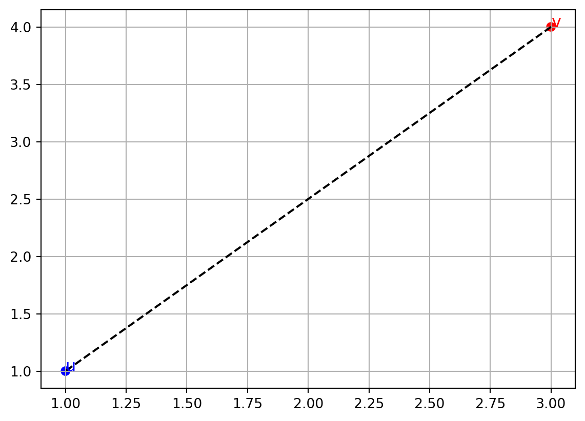
The dashed line shows the distance between the two points.

Higher-dimensional vectors Norms and distances work the same way in any dimension:

= np.array([1,2,3])
= np.array([4,0,8])
print("‖a‖ =", np.linalg.norm(a))
print("‖b‖ =", np.linalg.norm(b))
print("Distance between a and b =", np.linalg.norm(a-b))

‖a‖ = 3.7416573867739413
‖b‖ = 8.94427190999916
Distance between a and b = 6.164414002968976

Even though we can’t draw 3D easily on paper, the formulas still apply.

Try It Yourself

Compute the length of np.array([5,12]). What do you expect?
Find the distance between (2,3) and (7,7). Can you sketch it by hand and check?
In 3D, try vectors (1,1,1) and (2,2,2). Why is the distance exactly sqrt(3)?

6. Dot Product

The dot product is one of the most important operations in linear algebra. It takes two vectors and gives you a single number. That number combines both the lengths of the vectors and how much they point in the same direction. In this lab, we’ll calculate dot products in several ways, see how they relate to geometry, and visualize their meaning.

Set Up Your Lab

import numpy as np
import matplotlib.pyplot as plt

Step-by-Step Code Walkthrough

Algebraic definition The dot product of two vectors is the sum of the products of their components:

= np.array([2, 3])
= np.array([4, -1])

= v[0]*u[0] + v[1]*u[1]
= np.dot(v, u)

print("Manual dot product:", dot_manual)
print("NumPy dot product:", dot_numpy)

Manual dot product: 5
NumPy dot product: 5

Here, (2*4) + (3*-1) = 8 - 3 = 5.

Geometric definition The dot product also equals the product of the lengths of the vectors times the cosine of the angle between them:

\[
v \cdot u = \|v\| \|u\| \cos \theta
\]

We can compute the angle:

= np.linalg.norm(v)
= np.linalg.norm(u)

= np.dot(v, u) / (norm_v * norm_u)
= np.arccos(cos_theta)

print("cos(theta) =", cos_theta)
print("theta (in radians) =", theta)
print("theta (in degrees) =", np.degrees(theta))

cos(theta) = 0.33633639699815626
theta (in radians) = 1.2277723863741932
theta (in degrees) = 70.3461759419467

This gives the angle between v and u.

Visualizing the dot product Let’s draw the two vectors:

0,0,v[0],v[1],angles='xy',scale_units='xy',scale=1,color='r',label='v')
0,0,u[0],u[1],angles='xy',scale_units='xy',scale=1,color='b',label='u')
-1,5)
-2,4)
0,color='black',linewidth=0.5)
0,color='black',linewidth=0.5)

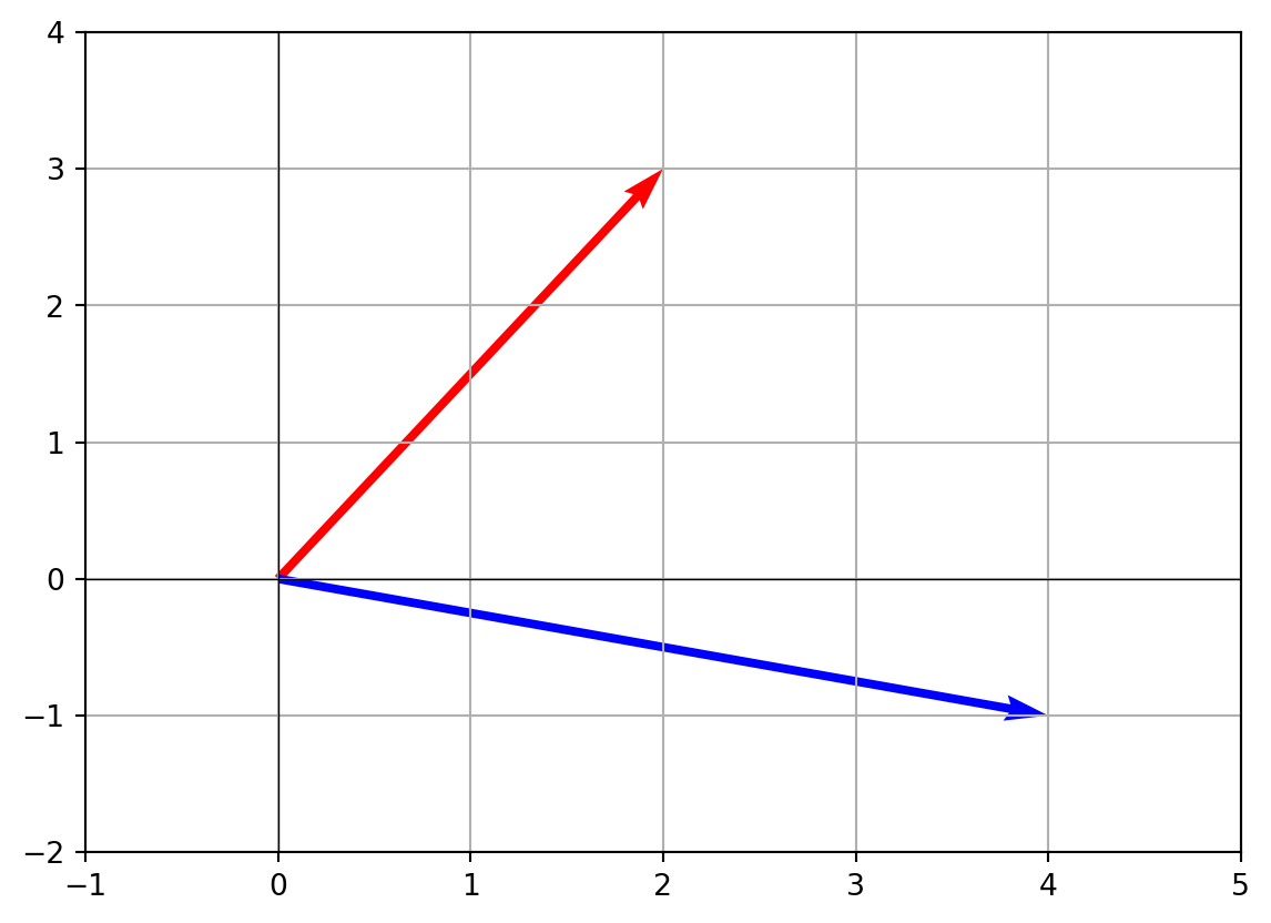
The dot product is positive if the angle is less than 90°, negative if greater than 90°, and zero if the vectors are perpendicular.

Projections and dot product The dot product lets us compute how much of one vector lies in the direction of another.

= np.dot(v, u) / np.linalg.norm(u)
print("Projection length of v onto u:", proj_length)

Projection length of v onto u: 1.212678125181665

This is the length of the shadow of v onto u.

Special cases

If vectors point in the same direction, the dot product is large and positive.
If vectors are perpendicular, the dot product is zero.
If vectors point in opposite directions, the dot product is negative.

= np.array([1,0])
= np.array([0,1])
= np.array([-1,0])

print("a · b =", np.dot(a,b))   # perpendicular
print("a · a =", np.dot(a,a))   # length squared
print("a · c =", np.dot(a,c))   # opposite

a · b = 0
a · a = 1
a · c = -1

Try It Yourself

Compute the dot product of (3,4) with (4,3). Is the result larger or smaller than the product of their lengths?
Try (1,2,3) · (4,5,6). Does the geometric meaning still work in 3D?
Create two perpendicular vectors (e.g. (2,0) and (0,5)). Verify the dot product is zero.

7. Angles Between Vectors and Cosine

In this lab, we’ll go deeper into the connection between vectors and geometry by calculating angles. Angles tell us how much two vectors “point in the same direction.” The bridge between algebra and geometry here is the cosine formula, which comes directly from the dot product.

Set Up Your Lab

import numpy as np
import matplotlib.pyplot as plt

Step-by-Step Code Walkthrough

Formula for the angle The angle \(\theta\) between two vectors \(v\) and \(u\) is given by:

\[
\cos \theta = \frac{v \cdot u}{\|v\| \, \|u\|}
\]

This means:

If \(\cos \theta = 1\), the vectors point in exactly the same direction.
If \(\cos \theta = 0\), they are perpendicular.
If \(\cos \theta = -1\), they point in opposite directions.

Computing the angle in Python

= np.array([2, 3])
= np.array([3, -1])

= np.dot(v, u)
= np.linalg.norm(v)
= np.linalg.norm(u)

= dot / (norm_v * norm_u)
= np.arccos(cos_theta)

print("cos(theta) =", cos_theta)
print("theta in radians =", theta)
print("theta in degrees =", np.degrees(theta))

cos(theta) = 0.2631174057921088
theta in radians = 1.3045442776439713
theta in degrees = 74.74488129694222

This gives both the cosine value and the actual angle.

Visualizing the vectors

0,0,v[0],v[1],angles='xy',scale_units='xy',scale=1,color='r',label='v')
0,0,u[0],u[1],angles='xy',scale_units='xy',scale=1,color='b',label='u')

-1,4)
-2,4)
0,color='black',linewidth=0.5)
0,color='black',linewidth=0.5)

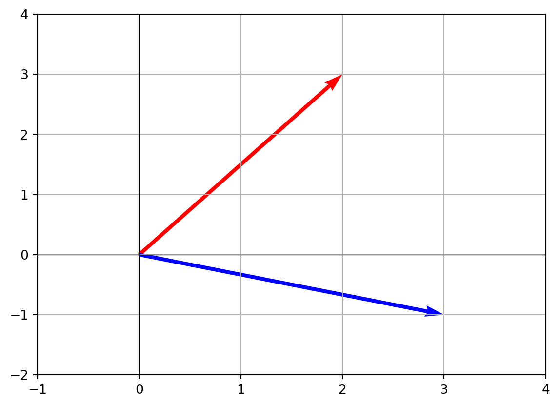
You can see the angle between v and u as the gap between the red and blue arrows.

Checking special cases

= np.array([1,0])
= np.array([0,1])
= np.array([-1,0])

print("Angle between a and b =", np.degrees(np.arccos(np.dot(a,b)/(np.linalg.norm(a)*np.linalg.norm(b)))))
print("Angle between a and c =", np.degrees(np.arccos(np.dot(a,c)/(np.linalg.norm(a)*np.linalg.norm(c)))))

Angle between a and b = 90.0
Angle between a and c = 180.0

Angle between (1,0) and (0,1) is 90°.
Angle between (1,0) and (-1,0) is 180°.

Using cosine as a similarity measure In data science and machine learning, people often use cosine similarity instead of raw angles. It’s just the cosine value itself:

= np.dot(v,u)/(np.linalg.norm(v)*np.linalg.norm(u))
print("Cosine similarity =", cosine_similarity)

Cosine similarity = 0.2631174057921088

Values close to 1 mean vectors are aligned, values near 0 mean unrelated, and values near -1 mean opposite.

Try It Yourself

Create two random vectors with np.random.randn(3) and compute the angle between them.
Verify that swapping the vectors gives the same angle (symmetry).
Find two vectors where cosine similarity is exactly 0. Can you come up with an example in 2D?

8. Projections and Decompositions

In this lab, we’ll learn how to split one vector into parts: one part that lies along another vector, and one part that is perpendicular. This process is called projection and decomposition. Projections let us measure “how much of a vector points in a given direction,” and decompositions give us a way to break vectors into useful components.

Set Up Your Lab

import numpy as np
import matplotlib.pyplot as plt

Step-by-Step Code Walkthrough

Projection formula The projection of vector \(v\) onto vector \(u\) is:

\[
\text{proj}_u(v) = \frac{v \cdot u}{u \cdot u} \, u
\]

This gives the component of \(v\) that points in the direction of \(u\).

Computing projection in Python

= np.array([3, 2])
= np.array([2, 0])

= (np.dot(v, u) / np.dot(u, u)) * u
print("Projection of v onto u:", proj_u_v)

Projection of v onto u: [3. 0.]

Here, \(v = (3,2)\) and \(u = (2,0)\). The projection of v onto u is a vector pointing along the x-axis.

Decomposing into parallel and perpendicular parts

We can write:

\[
v = \text{proj}_u(v) + (v – \text{proj}_u(v))
\]

The first part is parallel to u, the second part is perpendicular.

= v - proj_u_v
print("Parallel part:", proj_u_v)
print("Perpendicular part:", perp)

Parallel part: [3. 0.]
Perpendicular part: [0. 2.]

Visualizing projection and decomposition

0, 0, v[0], v[1], angles='xy', scale_units='xy', scale=1, color='r', label='v')
0, 0, u[0], u[1], angles='xy', scale_units='xy', scale=1, color='b', label='u')
0, 0, proj_u_v[0], proj_u_v[1], angles='xy', scale_units='xy', scale=1, color='g', label='proj_u(v)')
0], proj_u_v[1], perp[0], perp[1], angles='xy', scale_units='xy', scale=1, color='m', label='perpendicular')

-1, 5)
-1, 4)
0, color='black', linewidth=0.5)
0, color='black', linewidth=0.5)

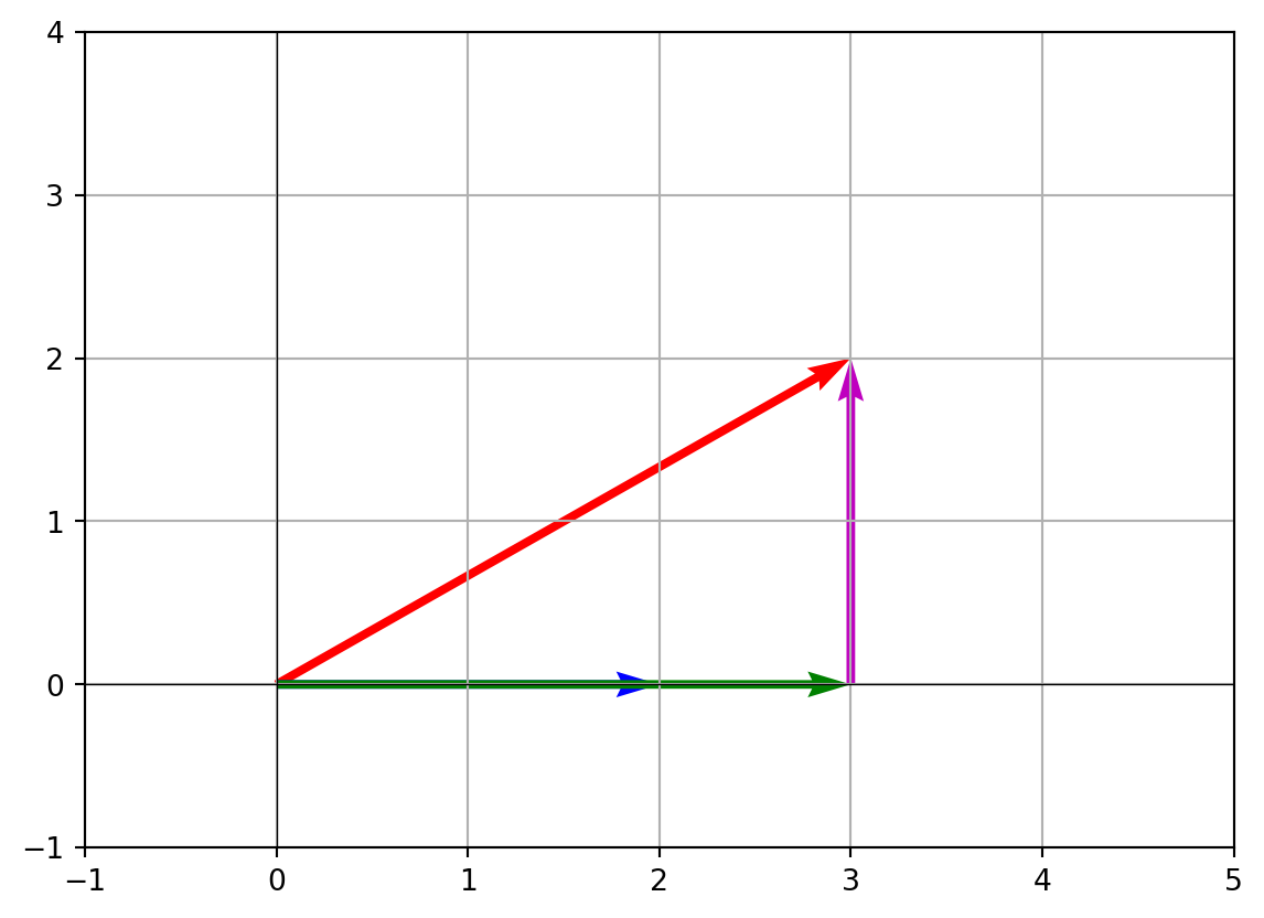
You’ll see v (red), u (blue), the projection (green), and the perpendicular remainder (magenta).

Projection in higher dimensions

This formula works in any dimension:

= np.array([1,2,3])
= np.array([0,1,0])

= (np.dot(a,b)/np.dot(b,b)) * b
= a - proj

print("Projection of a onto b:", proj)
print("Perpendicular component:", perp)

Projection of a onto b: [0. 2. 0.]
Perpendicular component: [1. 0. 3.]

Even in 3D or higher, projections are about splitting into “along” and “across.”

Try It Yourself

Try projecting (2,3) onto (0,5). Where does it land?
Take a 3D vector like (4,2,6) and project it onto (1,0,0). What does this give you?
Change the base vector u to something not aligned with the axes, like (1,1). Does the projection still work?

9. Cauchy–Schwarz and Triangle Inequalities

This lab introduces two fundamental inequalities in linear algebra. They may look abstract at first, but they provide guarantees that always hold true for vectors. We’ll explore them with small examples in Python to see why they matter.

Set Up Your Lab

import numpy as np

Step-by-Step Code Walkthrough

Cauchy–Schwarz inequality

The inequality states:

\[
|v \cdot u| \leq \|v\| \, \|u\|
\]

It means the dot product is never “bigger” than the product of the vector lengths. Equality happens only if the two vectors are pointing in exactly the same (or opposite) direction.

= np.array([3, 4])
= np.array([1, 2])

= abs(np.dot(v, u))
= np.linalg.norm(v) * np.linalg.norm(u)

print("Left-hand side (|v·u|):", lhs)
print("Right-hand side (‖v‖‖u‖):", rhs)
print("Inequality holds?", lhs <= rhs)

Left-hand side (|v·u|): 11
Right-hand side (‖v‖‖u‖): 11.180339887498949
Inequality holds? True

Testing Cauchy–Schwarz with different vectors

= [
1,0]), np.array([0,1])),  # perpendicular
2,3]), np.array([4,6])),  # multiples
-1,2]), np.array([3,-6])) # opposite multiples


for v,u in pairs:
= abs(np.dot(v, u))
= np.linalg.norm(v) * np.linalg.norm(u)
print(f"v={v}, u={u} -> |v·u|={lhs}, ‖v‖‖u‖={rhs}, holds={lhs<=rhs}")

v=[1 0], u=[0 1] -> |v·u|=0, ‖v‖‖u‖=1.0, holds=True
v=[2 3], u=[4 6] -> |v·u|=26, ‖v‖‖u‖=25.999999999999996, holds=False
v=[-1  2], u=[ 3 -6] -> |v·u|=15, ‖v‖‖u‖=15.000000000000002, holds=True

Perpendicular vectors give |v·u| = 0, far less than the product of norms.
Multiples give equality (lhs = rhs).

Triangle inequality

The triangle inequality states:

\[
\|v + u\| \leq \|v\| + \|u\|
\]

Geometrically, the length of one side of a triangle can never be longer than the sum of the other two sides.

= np.array([3, 4])
= np.array([1, 2])

= np.linalg.norm(v + u)
= np.linalg.norm(v) + np.linalg.norm(u)

print("‖v+u‖ =", lhs)
print("‖v‖ + ‖u‖ =", rhs)
print("Inequality holds?", lhs <= rhs)

‖v+u‖ = 7.211102550927978
‖v‖ + ‖u‖ = 7.23606797749979
Inequality holds? True

Visual demonstration with a triangle

import matplotlib.pyplot as plt

= np.array([0,0])
= np.array([origin, v, v+u, origin])

0], points[:,1], 'ro-')  # triangle outline
0], v[1], 'v')
0]+u[0], v[1]+u[1], 'v+u')
0], u[1], 'u')


0,color='black',linewidth=0.5)
0,color='black',linewidth=0.5)
'equal')

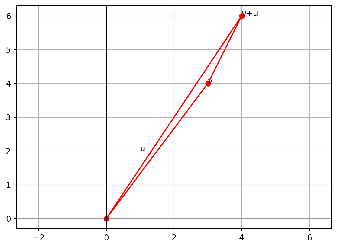
This triangle shows why the inequality is called the “triangle” inequality.

Testing triangle inequality with random vectors

for _ in range(5):
= np.random.randn(2)
= np.random.randn(2)
= np.linalg.norm(v+u)
= np.linalg.norm(v) + np.linalg.norm(u)
print(f"‖v+u‖={lhs:.3f}, ‖v‖+‖u‖={rhs:.3f}, holds={lhs <= rhs}")

‖v+u‖=0.778, ‖v‖+‖u‖=2.112, holds=True
‖v+u‖=1.040, ‖v‖+‖u‖=2.621, holds=True
‖v+u‖=1.632, ‖v‖+‖u‖=2.482, holds=True
‖v+u‖=1.493, ‖v‖+‖u‖=2.250, holds=True
‖v+u‖=2.653, ‖v‖+‖u‖=2.692, holds=True

No matter what vectors you try, the inequality always holds.

The Takeaway

Cauchy–Schwarz: The dot product is always bounded by the product of vector lengths.
Triangle inequality: The length of one side of a triangle can’t exceed the sum of the other two.
These inequalities form the backbone of geometry, analysis, and many proofs in linear algebra.

10. Orthonormal Sets in ℝ²/ℝ³

In this lab, we’ll explore orthonormal sets – collections of vectors that are both orthogonal (perpendicular) and normalized (length = 1). These sets are the “nicest” possible bases for vector spaces. In 2D and 3D, they correspond to the coordinate axes we already know, but we can also construct and test new ones.

Set Up Your Lab

import numpy as np
import matplotlib.pyplot as plt

Step-by-Step Code Walkthrough

Orthogonal vectors Two vectors are orthogonal if their dot product is zero.

= np.array([1, 0])
= np.array([0, 1])

print("x_axis · y_axis =", np.dot(x_axis, y_axis))  # should be 0

x_axis · y_axis = 0

So the standard axes are orthogonal.

Normalizing vectors Normalization means dividing a vector by its length to make its norm equal to 1.

= np.array([3, 4])
= v / np.linalg.norm(v)

print("Original v:", v)
print("Normalized v:", v_normalized)
print("Length of normalized v:", np.linalg.norm(v_normalized))

Original v: [3 4]
Normalized v: [0.6 0.8]
Length of normalized v: 1.0

Now v_normalized points in the same direction as v but has unit length.

Building an orthonormal set in 2D

= np.array([1, 0])
= np.array([0, 1])

print("u1 length:", np.linalg.norm(u1))
print("u2 length:", np.linalg.norm(u2))
print("u1 · u2 =", np.dot(u1,u2))

u1 length: 1.0
u2 length: 1.0
u1 · u2 = 0

Both have length 1, and their dot product is 0. That makes {u1, u2} an orthonormal set in 2D.

Visualizing 2D orthonormal vectors

0,0,u1[0],u1[1],angles='xy',scale_units='xy',scale=1,color='r')
0,0,u2[0],u2[1],angles='xy',scale_units='xy',scale=1,color='b')

-1.5,1.5)
-1.5,1.5)
0,color='black',linewidth=0.5)
0,color='black',linewidth=0.5)

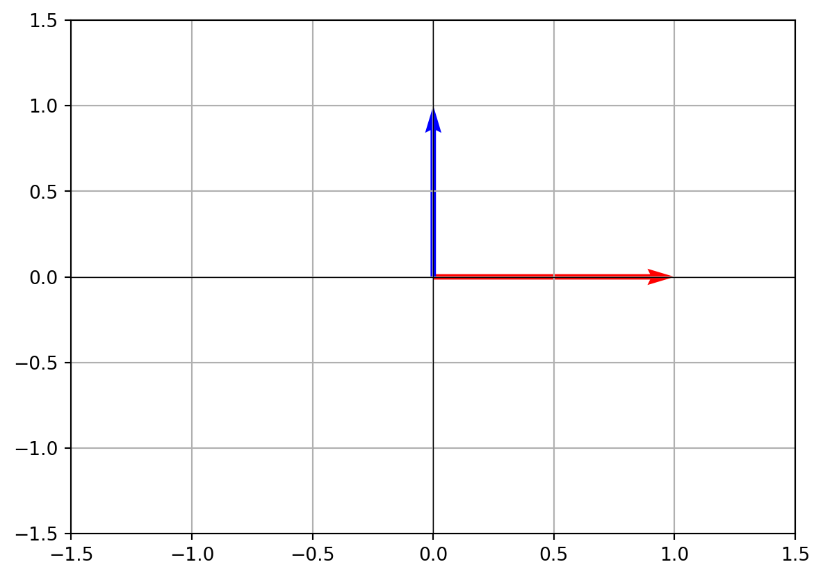
You’ll see the red and blue arrows at right angles, each of length 1.

Orthonormal set in 3D In 3D, the standard basis vectors are:

= np.array([1,0,0])
= np.array([0,1,0])
= np.array([0,0,1])

print("‖i‖ =", np.linalg.norm(i))
print("‖j‖ =", np.linalg.norm(j))
print("‖k‖ =", np.linalg.norm(k))
print("i·j =", np.dot(i,j))
print("j·k =", np.dot(j,k))
print("i·k =", np.dot(i,k))

‖i‖ = 1.0
‖j‖ = 1.0
‖k‖ = 1.0
i·j = 0
j·k = 0
i·k = 0

Lengths are all 1, and dot products are 0. So {i, j, k} is an orthonormal set in ℝ³.

Testing if a set is orthonormal We can write a helper function:

def is_orthonormal(vectors):
for i in range(len(vectors)):
for j in range(len(vectors)):
= np.dot(vectors[i], vectors[j])
if i == j:
if not np.isclose(dot, 1): return False
else:
if not np.isclose(dot, 0): return False
return True

print(is_orthonormal([i, j, k]))  # True

True

Constructing a new orthonormal pair Not all orthonormal sets look like the axes.

= np.array([1,1]) / np.sqrt(2)
= np.array([-1,1]) / np.sqrt(2)

print("u1·u2 =", np.dot(u1,u2))
print("‖u1‖ =", np.linalg.norm(u1))
print("‖u2‖ =", np.linalg.norm(u2))

u1·u2 = 0.0
‖u1‖ = 0.9999999999999999
‖u2‖ = 0.9999999999999999

This gives a rotated orthonormal basis in 2D.

Try It Yourself

Normalize (2,2,1) to make it a unit vector.
Test whether the set {[1,0,0], [0,2,0], [0,0,3]} is orthonormal.
Construct two vectors in 2D that are not perpendicular. Normalize them and check if the dot product is still zero.

Chapter 2. Matrices and basic operations

11. Matrices as Tables and as Machines

Matrices can feel mysterious at first, but there are two simple ways to think about them:

As tables of numbers – just a grid you can store and manipulate.
As machines – something that takes a vector in and spits a new vector out.

In this lab, we’ll explore both views and see how they connect.

Set Up Your Lab

import numpy as np

Step-by-Step Code Walkthrough

A matrix as a table of numbers

= np.array([
1, 2, 3],
4, 5, 6]


print("Matrix A:\n", A)
print("Shape of A:", A.shape)

Matrix A:
 [[1 2 3]
 [4 5 6]]
Shape of A: (2, 3)

Here, A is a 2×3 matrix (2 rows, 3 columns).

Rows = horizontal slices → [1,2,3] and [4,5,6]
Columns = vertical slices → [1,4], [2,5], [3,6]

Accessing rows and columns

= A[0]        # row 0
= A[:,1]  # column 1

print("First row:", first_row)
print("Second column:", second_column)

First row: [1 2 3]
Second column: [2 5]

Rows are whole vectors too, and so are columns.

A matrix as a machine

A matrix can “act” on a vector. If x = [x1, x2, x3], then A·x is computed by taking linear combinations of the columns of A.

= np.array([1, 0, -1])  # a 3D vector
= A.dot(x)

print("A·x =", result)

A·x = [-2 -2]

Interpretation: multiply A by x = combine columns of A with weights from x.

\[
A \cdot x = 1 \cdot \text{(col 1)} + 0 \cdot \text{(col 2)} + (-1) \cdot \text{(col 3)}
\]

Verifying column combination view

= A[:,0]
= A[:,1]
= A[:,2]

= 1*col1 + 0*col2 + (-1)*col3
print("Manual combination:", manual)
print("A·x result:", result)

Manual combination: [-2 -2]
A·x result: [-2 -2]

They match exactly. This shows the “machine” interpretation is just a shortcut for column combinations.

Geometric intuition (2D example)

= np.array([
2, 0],
0, 1]


= np.array([1,2])
print("B·v =", B.dot(v))

B·v = [2 2]

Here, B scales the x-direction by 2 while leaving the y-direction alone. So (1,2) becomes (2,2).

Try It Yourself

Create a 3×3 identity matrix with np.eye(3) and multiply it by different vectors. What happens?
Build a matrix [[0,-1],[1,0]]. Try multiplying it by (1,0) and (0,1). What transformation is this?
Create your own 2×2 matrix that flips vectors across the x-axis. Test it on (1,2) and (−3,4).

The Takeaway

A matrix is both a grid of numbers and a machine that transforms vectors.
Matrix–vector multiplication is the same as combining columns with given weights.
Thinking of matrices as machines helps build intuition for rotations, scalings, and other transformations later.

12. Matrix Shapes, Indexing, and Block Views

Matrices come in many shapes, and learning to read their structure is essential. Shape tells us how many rows and columns a matrix has. Indexing lets us grab specific entries, rows, or columns. Block views let us zoom in on submatrices, which is extremely useful for both theory and computation.

Set Up Your Lab

import numpy as np

Step-by-Step Code Walkthrough

Matrix shapes

The shape of a matrix is (rows, columns).

= np.array([
1, 2, 3],
4, 5, 6],
7, 8, 9]


print("Matrix A:\n", A)
print("Shape of A:", A.shape)

Matrix A:
 [[1 2 3]
 [4 5 6]
 [7 8 9]]
Shape of A: (3, 3)

Here, A is a 3×3 matrix.

Indexing elements

In NumPy, rows and columns are 0-based. The first entry is A[0,0].

print("A[0,0] =", A[0,0])  # top-left element
print("A[1,2] =", A[1,2])  # second row, third column

A[0,0] = 1
A[1,2] = 6

Extracting rows and columns

= A[0]       # first row
= A[:,1]     # second column

print("First row:", row1)
print("Second column:", col2)

First row: [1 2 3]
Second column: [2 5 8]

Notice: A[i] gives a row, A[:,j] gives a column.

Slicing submatrices (block view)

You can slice multiple rows and columns to form a smaller matrix.

= A[0:2, 1:3]  # rows 0–1, columns 1–2
print("Block submatrix:\n", block)

Block submatrix:
 [[2 3]
 [5 6]]

This block is:

\[
\begin{bmatrix}
2 & 3 \\
5 & 6
\end{bmatrix}
\]

Modifying parts of a matrix

0,0] = 99
print("Modified A:\n", A)

1,:] = [10, 11, 12]   # replace row 1
print("After replacing row 1:\n", A)

Modified A:
 [[99  2  3]
 [ 4  5  6]
 [ 7  8  9]]
After replacing row 1:
 [[99  2  3]
 [10 11 12]
 [ 7  8  9]]

Non-square matrices

Not all matrices are square. Shapes can be rectangular, too.

= np.array([
1, 2],
3, 4],
5, 6]


print("Matrix B:\n", B)
print("Shape of B:", B.shape)

Matrix B:
 [[1 2]
 [3 4]
 [5 6]]
Shape of B: (3, 2)

Here, B is 3×2 (3 rows, 2 columns).

Block decomposition idea

We can think of large matrices as made of smaller blocks. This is common in linear algebra proofs and algorithms.

= np.array([
1,2,3,4],
5,6,7,8],
9,10,11,12],
13,14,15,16]


= C[0:2, 0:2]
= C[2:4, 2:4]

print("Top-left block:\n", top_left)
print("Bottom-right block:\n", bottom_right)

Top-left block:
 [[1 2]
 [5 6]]
Bottom-right block:
 [[11 12]
 [15 16]]

This is the start of block matrix notation.

Try It Yourself

Create a 4×5 matrix with values 1–20 using np.arange(1,21).reshape(4,5). Find its shape.
Extract the middle row and last column.
Cut it into four 2×2 blocks. Can you reassemble them in a different order?

13. Matrix Addition and Scalar Multiplication

Now that we understand matrix shapes and indexing, let’s practice two of the simplest but most important operations: adding matrices and scaling them with numbers (scalars). These operations extend the rules we already know for vectors.

Set Up Your Lab

import numpy as np

Step-by-Step Code Walkthrough

Adding two matrices You can add two matrices if (and only if) they have the same shape. Addition happens entry by entry.

= np.array([
1, 2],
3, 4]


= np.array([
5, 6],
7, 8]


= A + B
print("A + B =\n", C)

A + B =
 [[ 6  8]
 [10 12]]

Each element in C is the sum of corresponding elements in A and B.

Scalar multiplication Multiplying a matrix by a scalar multiplies every entry by that number.

= 3
= k * A
print("3 * A =\n", D)

3 * A =
 [[ 3  6]
 [ 9 12]]

Here, each element of A is tripled.

Combining both operations We can mix addition and scaling, just like with vectors.

= 2*A - B
print("2A - B =\n", combo)

2A - B =
 [[-3 -2]
 [-1  0]]

This creates new matrices as linear combinations of others.

Zero matrix A matrix of all zeros acts like “nothing happens” for addition.

= np.zeros((2,2))
print("Zero matrix:\n", zero)
print("A + Zero =\n", A + zero)

Zero matrix:
 [[0. 0.]
 [0. 0.]]
A + Zero =
 [[1. 2.]
 [3. 4.]]

Shape mismatch (what fails) If shapes don’t match, NumPy throws an error.

= np.array([
1,2,3],
4,5,6]


try:
print(A + X)
except ValueError as e:
print("Error:", e)

Error: operands could not be broadcast together with shapes (2,2) (2,3)

This shows why shape consistency matters.

Try It Yourself

Create two random 3×3 matrices with np.random.randint(0,10,(3,3)) and add them.
Multiply a 4×4 matrix by -1. What happens to its entries?
Compute 3A + 2B with the matrices from above. Compare with doing each step manually.

14. Matrix–Vector Product (Linear Combinations of Columns)

This lab introduces the matrix–vector product, one of the most important operations in linear algebra. Multiplying a matrix by a vector doesn’t just crunch numbers – it produces a new vector by combining the matrix’s columns in a weighted way.

Set Up Your Lab

import numpy as np

Step-by-Step Code Walkthrough

A simple matrix and vector

= np.array([
1, 2],
3, 4],
5, 6]
# 3×2 matrix

= np.array([2, -1])  # 2D vector

Here, A has 2 columns, so we can multiply it by a 2D vector x.

Matrix–vector multiplication in NumPy

= A.dot(x)
print("A·x =", y)

A·x = [0 2 4]

Result: a 3D vector.

Interpreting the result as linear combinations

Matrix A has two columns:

= A[:,0]   # first column
= A[:,1]   # second column

= 2*col1 + (-1)*col2
print("Manual linear combination:", manual)

Manual linear combination: [0 2 4]

This matches A·x. In words: multiply each column by the corresponding entry of x and then add them up.

Another example (geometry)

= np.array([
2, 0],
0, 1]
# stretches x-axis by 2

= np.array([1, 3])
print("B·v =", B.dot(v))

B·v = [2 3]

Here, (1,3) becomes (2,3). The x-component was doubled, while y stayed the same.

Visualization of matrix action

import matplotlib.pyplot as plt

# draw original vector
0,0,v[0],v[1],angles='xy',scale_units='xy',scale=1,color='r',label='v')

# draw transformed vector
= B.dot(v)
0,0,v_transformed[0],v_transformed[1],angles='xy',scale_units='xy',scale=1,color='b',label='B·v')

-1,4)
-1,4)
0,color='black',linewidth=0.5)
0,color='black',linewidth=0.5)

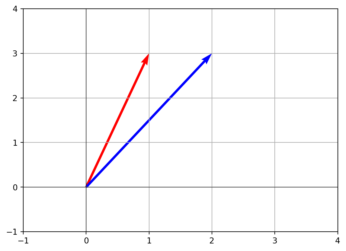
Red arrow = original vector, blue arrow = transformed vector.

Try It Yourself

Multiply

\[
A = \begin{bmatrix}1 & 0 \\ 0 & 1 \\ -1 & 2\end{bmatrix},\; x = [3,1]
\]

What’s the result?
Replace B with [[0,-1],[1,0]]. Multiply it by (1,0) and (0,1). What geometric transformation does this represent?
For a 4×4 identity matrix (np.eye(4)), try multiplying by any 4D vector. What do you observe?

15. Matrix–Matrix Product (Composition of Linear Steps)

Matrix–matrix multiplication is how we combine two linear transformations into one. Instead of applying one transformation, then another, we can multiply their matrices and get a single matrix that does both at once.

Set Up Your Lab

import numpy as np

Step-by-Step Code Walkthrough

Matrix–matrix multiplication in NumPy

= np.array([
1, 2],
3, 4]
# 2×2

= np.array([
2, 0],
1, 2]
# 2×2

= A.dot(B)   # or A @ B
print("A·B =\n", C)

A·B =
 [[ 4  4]
 [10  8]]

The result C is another 2×2 matrix.

Manual computation

Each entry of C is computed as a row of A dotted with a column of B:

= A[0,:].dot(B[:,0])
= A[0,:].dot(B[:,1])
= A[1,:].dot(B[:,0])
= A[1,:].dot(B[:,1])

print("Manual C =\n", np.array([[c11,c12],[c21,c22]]))

Manual C =
 [[ 4  4]
 [10  8]]

This should match A·B.

Geometric interpretation

Let’s see how two transformations combine.

Matrix B scales x by 2 and stretches y by 2.
Matrix A applies another linear transformation.

Together, C = A·B does both in one step.

= np.array([1,1])

print("First apply B:", B.dot(v))
print("Then apply A:", A.dot(B.dot(v)))
print("Directly with C:", C.dot(v))

First apply B: [2 3]
Then apply A: [ 8 18]
Directly with C: [ 8 18]

The result is the same: applying B then A is equivalent to applying C.

Non-square matrices

Matrix multiplication also works for rectangular matrices, as long as the inner dimensions match.

= np.array([
1, 0, 2],
0, 1, 3]
# 2×3

= np.array([
1, 2],
0, 1],
4, 0]
# 3×2

= M.dot(N)  # result is 2×2
print("M·N =\n", P)

M·N =
 [[ 9  2]
 [12  1]]

Shape rule: (2×3)·(3×2) = (2×2).

Associativity (but not commutativity)

Matrix multiplication is associative: (A·B)·C = A·(B·C). But it’s not commutative: in general, A·B ≠ B·A.

= np.array([[1,2],[3,4]])
= np.array([[0,1],[1,0]])

print("A·B =\n", A.dot(B))
print("B·A =\n", B.dot(A))

A·B =
 [[2 1]
 [4 3]]
B·A =
 [[3 4]
 [1 2]]

The two results are different.

Try It Yourself

Multiply

\[
A = \begin{bmatrix}1 & 0 \\ 0 & 1\end{bmatrix},\;
B = \begin{bmatrix}0 & -1 \\ 1 & 0\end{bmatrix}
\]

What transformation does A·B represent?
Create a random 3×2 matrix and a 2×4 matrix. Multiply them. What shape is the result?
Verify with Python that (A·B)·C = A·(B·C) for some 3×3 random matrices.

16. Identity, Inverse, and Transpose

In this lab, we’ll meet three special matrix operations and objects: the identity matrix, the inverse, and the transpose. These are the building blocks of matrix algebra, each with a simple meaning but deep importance.

Set Up Your Lab

import numpy as np

Step-by-Step Code Walkthrough

Identity matrix The identity matrix is like the number 1 for matrices: multiplying by it changes nothing.

= np.eye(3)  # 3×3 identity matrix
print("Identity matrix:\n", I)

= np.array([
2, 1, 0],
0, 1, 3],
4, 0, 1]


print("A·I =\n", A.dot(I))
print("I·A =\n", I.dot(A))

Identity matrix:
 [[1. 0. 0.]
 [0. 1. 0.]
 [0. 0. 1.]]
A·I =
 [[2. 1. 0.]
 [0. 1. 3.]
 [4. 0. 1.]]
I·A =
 [[2. 1. 0.]
 [0. 1. 3.]
 [4. 0. 1.]]

Both equal A.

Transpose The transpose flips rows and columns.

= np.array([
1, 2, 3],
4, 5, 6]


print("B:\n", B)
print("B.T:\n", B.T)

B:
 [[1 2 3]
 [4 5 6]]
B.T:
 [[1 4]
 [2 5]
 [3 6]]

Original: 2×3
Transpose: 3×2

Geometrically, transpose swaps the axes when vectors are viewed in row/column form.

Inverse The inverse matrix is like dividing by a number: multiplying a matrix by its inverse gives the identity.

= np.array([
2, 1],
5, 3]


= np.linalg.inv(C)
print("Inverse of C:\n", C_inv)

print("C·C_inv =\n", C.dot(C_inv))
print("C_inv·C =\n", C_inv.dot(C))

Inverse of C:
 [[ 3. -1.]
 [-5.  2.]]
C·C_inv =
 [[ 1.00000000e+00  2.22044605e-16]
 [-8.88178420e-16  1.00000000e+00]]
C_inv·C =
 [[1.00000000e+00 3.33066907e-16]
 [0.00000000e+00 1.00000000e+00]]

Both products are (approximately) the identity.

Matrices that don’t have inverses Not every matrix is invertible. If a matrix is singular (determinant = 0), it has no inverse.

= np.array([
1, 2],
2, 4]


try:

except np.linalg.LinAlgError as e:
print("Error:", e)

Error: Singular matrix

Here, the second row is a multiple of the first, so D can’t be inverted.

Transpose and inverse together For invertible matrices,

\[
(A^T)^{-1} = (A^{-1})^T
\]

We can check this numerically:

= np.array([
1, 2],
3, 5]


= np.linalg.inv(A.T)
= np.linalg.inv(A).T

print("Do they match?", np.allclose(lhs, rhs))

Do they match? True

Try It Yourself

Create a 4×4 identity matrix. Multiply it by any 4×1 vector. Does it change?
Take a random 2×2 matrix with np.random.randint. Compute its inverse and check if multiplying gives identity.
Pick a rectangular 3×2 matrix. What happens when you try np.linalg.inv? Why?
Compute (A.T).T for some matrix A. What do you notice?

17. Symmetric, Diagonal, Triangular, and Permutation Matrices

In this lab, we’ll meet four important families of special matrices. They have patterns that make them easier to understand, compute with, and use in algorithms.

Set Up Your Lab

import numpy as np

Step-by-Step Code Walkthrough

Symmetric matrices A matrix is symmetric if it equals its transpose: \(A = A^T\).

= np.array([
2, 3, 4],
3, 5, 6],
4, 6, 8]


print("A:\n", A)
print("A.T:\n", A.T)
print("Is symmetric?", np.allclose(A, A.T))

A:
 [[2 3 4]
 [3 5 6]
 [4 6 8]]
A.T:
 [[2 3 4]
 [3 5 6]
 [4 6 8]]
Is symmetric? True

Symmetric matrices appear in physics, optimization, and statistics (e.g., covariance matrices).

Diagonal matrices A diagonal matrix has nonzero entries only on the main diagonal.

= np.diag([1, 5, 9])
print("Diagonal matrix:\n", D)

= np.array([2, 3, 4])
print("D·x =", D.dot(x))  # scales each component

Diagonal matrix:
 [[1 0 0]
 [0 5 0]
 [0 0 9]]
D·x = [ 2 15 36]

Diagonal multiplication simply scales each coordinate separately.

Triangular matrices Upper triangular: all entries below the diagonal are zero. Lower triangular: all entries above the diagonal are zero.

= np.array([
1, 2, 3],
0, 4, 5],
0, 0, 6]


= np.array([
7, 0, 0],
8, 9, 0],
1, 2, 3]


print("Upper triangular U:\n", U)
print("Lower triangular L:\n", L)

Upper triangular U:
 [[1 2 3]
 [0 4 5]
 [0 0 6]]
Lower triangular L:
 [[7 0 0]
 [8 9 0]
 [1 2 3]]

These are important in solving linear systems (e.g., Gaussian elimination).

Permutation matrices A permutation matrix rearranges the order of coordinates. Each row and each column has exactly one 1, everything else is 0.

= np.array([
0, 1, 0],
0, 0, 1],
1, 0, 0]


print("Permutation matrix P:\n", P)

= np.array([10, 20, 30])
print("P·v =", P.dot(v))

Permutation matrix P:
 [[0 1 0]
 [0 0 1]
 [1 0 0]]
P·v = [20 30 10]

Here, P cycles (10,20,30) into (20,30,10).

Checking properties

def is_symmetric(M): return np.allclose(M, M.T)
def is_diagonal(M): return np.count_nonzero(M - np.diag(np.diag(M))) == 0
def is_upper_triangular(M): return np.allclose(M, np.triu(M))
def is_lower_triangular(M): return np.allclose(M, np.tril(M))

print("A symmetric?", is_symmetric(A))
print("D diagonal?", is_diagonal(D))
print("U upper triangular?", is_upper_triangular(U))
print("L lower triangular?", is_lower_triangular(L))

A symmetric? True
D diagonal? True
U upper triangular? True
L lower triangular? True

Try It Yourself

Create a random symmetric matrix by generating any matrix M and computing (M + M.T)/2.
Build a 4×4 diagonal matrix with diagonal entries [2,4,6,8] and multiply it by [1,1,1,1].
Make a permutation matrix that swaps the first and last components of a 3D vector.
Check whether the identity matrix is diagonal, symmetric, upper triangular, and lower triangular all at once.

18. Trace and Basic Matrix Properties

In this lab, we’ll introduce the trace of a matrix and a few quick properties that often appear in proofs, algorithms, and applications. The trace is simple to compute but surprisingly powerful.

Set Up Your Lab

import numpy as np

Step-by-Step Code Walkthrough

What is the trace? The trace of a square matrix is the sum of its diagonal entries:

\[
\text{tr}(A) = \sum_i A_{ii}
\]

= np.array([
2, 1, 3],
0, 4, 5],
7, 8, 6]


= np.trace(A)
print("Matrix A:\n", A)
print("Trace of A =", trace_A)

Matrix A:
 [[2 1 3]
 [0 4 5]
 [7 8 6]]
Trace of A = 12

Here, trace = \(2 + 4 + 6 = 12\).

Trace is linear For matrices A and B:

\[
\text{tr}(A+B) = \text{tr}(A) + \text{tr}(B)
\]

\[
\text{tr}(cA) = c \cdot \text{tr}(A)
\]

= np.array([
1, 0, 0],
0, 2, 0],
0, 0, 3]


print("tr(A+B) =", np.trace(A+B))
print("tr(A) + tr(B) =", np.trace(A) + np.trace(B))

print("tr(3A) =", np.trace(3*A))
print("3 * tr(A) =", 3*np.trace(A))

tr(A+B) = 18
tr(A) + tr(B) = 18
tr(3A) = 36
3 * tr(A) = 36

Trace of a product One important property is:

\[
\text{tr}(AB) = \text{tr}(BA)
\]

= np.array([
0,1],
2,3]


= np.array([
4,5],
6,7]


print("tr(CD) =", np.trace(C.dot(D)))
print("tr(DC) =", np.trace(D.dot(C)))

tr(CD) = 37
tr(DC) = 37

Both are equal, even though CD and DC are different matrices.

Trace and eigenvalues The trace equals the sum of eigenvalues of a matrix (counting multiplicities).

= np.linalg.eig(A)
print("Eigenvalues:", vals)
print("Sum of eigenvalues =", np.sum(vals))
print("Trace =", np.trace(A))

Eigenvalues: [12.83286783  2.13019807 -2.9630659 ]
Sum of eigenvalues = 12.000000000000007
Trace = 12

The results should match (within rounding error).

Quick invariants

Trace doesn’t change under transpose: tr(A) = tr(A.T)
Trace doesn’t change under similarity transforms: tr(P^-1 A P) = tr(A)

print("tr(A) =", np.trace(A))
print("tr(A.T) =", np.trace(A.T))

tr(A) = 12
tr(A.T) = 12

Try It Yourself

Create a 2×2 rotation matrix for 90°:

\[
R = \begin{bmatrix}0 & -1 \\ 1 & 0\end{bmatrix}
\]

What is its trace? What does that tell you about its eigenvalues?
Make a random 3×3 matrix and compare tr(A) with the sum of eigenvalues.
Test tr(AB) and tr(BA) with a rectangular matrix A (e.g. 2×3) and B (3×2). Do they still match?

19. Affine Transforms and Homogeneous Coordinates

Affine transformations let us do more than just linear operations – they include translations (shifting points), which ordinary matrices can’t handle alone. To unify rotations, scalings, reflections, and translations, we use homogeneous coordinates.

Set Up Your Lab

import numpy as np
import matplotlib.pyplot as plt

Step-by-Step Code Walkthrough

Linear transformations vs affine transformations

A linear transformation can rotate, scale, or shear, but always keeps the origin fixed.
An affine transformation allows translation as well.

For example, shifting every point by (2,3) is affine but not linear.

Homogeneous coordinates idea We add an extra coordinate (usually 1) to vectors.

A 2D point (x,y) becomes (x,y,1).
A 3D point (x,y,z) becomes (x,y,z,1).

This trick lets us represent translations using matrix multiplication.

2D translation matrix

\[
T = \begin{bmatrix}
1 & 0 & t_x \\
0 & 1 & t_y \\
0 & 0 & 1
\end{bmatrix}
\]

= np.array([
1, 0, 2],
0, 1, 3],
0, 0, 1]


= np.array([1, 1, 1])  # point at (1,1)
= T.dot(p)

print("Original point:", p)
print("Translated point:", p_translated)

Original point: [1 1 1]
Translated point: [3 4 1]

This shifts (1,1) to (3,4).

Combining rotation and translation

A 90° rotation around the origin in 2D:

= np.array([
0, -1, 0],
1,  0, 0],
0,  0, 1]


= T.dot(R)  # rotate then translate
print("Combined transform:\n", M)

= np.array([1, 0, 1])
print("Rotated + translated point:", M.dot(p))

Combined transform:
 [[ 0 -1  2]
 [ 1  0  3]
 [ 0  0  1]]
Rotated + translated point: [2 4 1]

Now we can apply rotation and translation in one step.

Visualization of translation

= np.array([
0,0,1],
1,0,1],
1,1,1],
0,1,1]
# a unit square

= points.dot(T.T)

0], points[:,1], color='r', label='original')
0], transformed[:,1], color='b', label='translated')

for i in range(len(points)):
0], points[i,1],
0]-points[i,0],
1]-points[i,1],
=0.05, color='gray')


'equal')

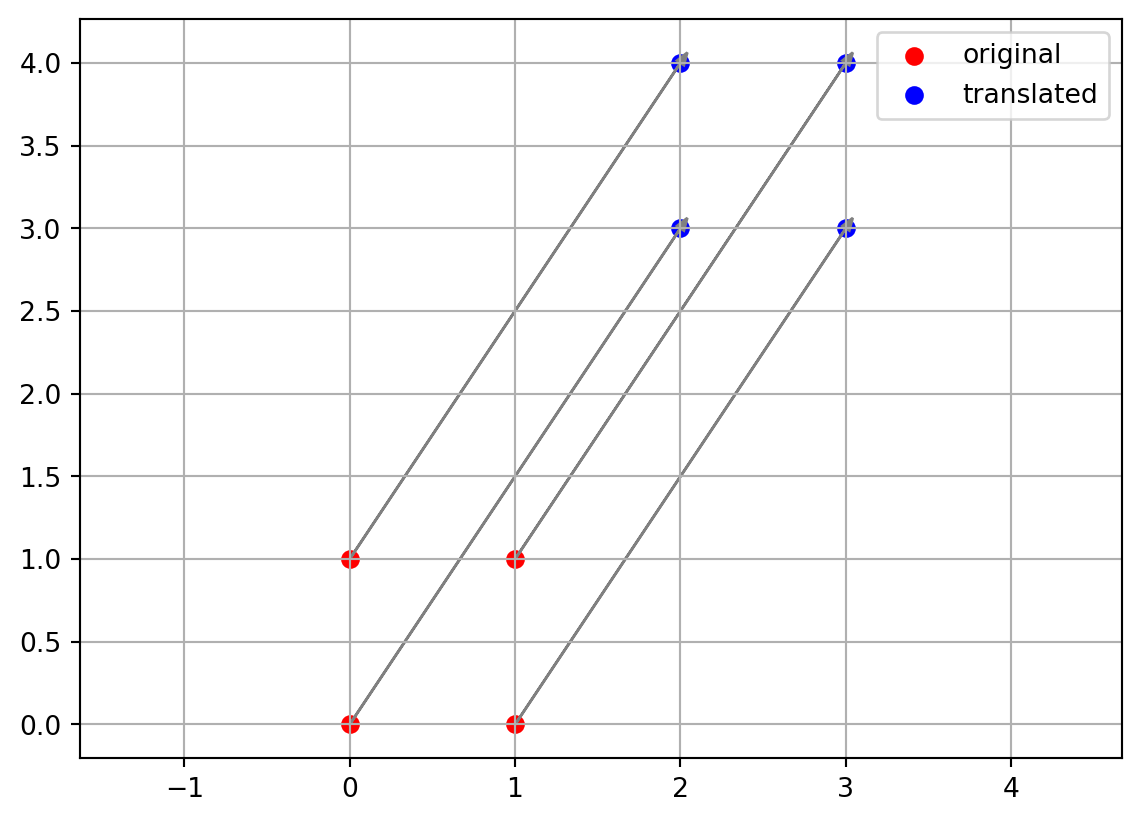
You’ll see the red unit square moved to a blue unit square shifted by (2,3).

Extending to 3D In 3D, homogeneous coordinates use 4×4 matrices. Translations, rotations, and scalings all fit the same framework.

= np.array([
1,0,0,5],
0,1,0,-2],
0,0,1,3],
0,0,0,1]


= np.array([1,2,3,1])
print("Translated 3D point:", T3.dot(p3))

Translated 3D point: [6 0 6 1]

This shifts (1,2,3) to (6,0,6).

Try It Yourself

Build a scaling matrix in homogeneous coordinates that doubles both x and y, and apply it to (1,1).
Create a 2D transform that rotates by 90° and then shifts by (−2,1). Apply it to (0,2).
In 3D, translate (0,0,0) by (10,10,10). What homogeneous matrix did you use?

20. Computing with Matrices (Cost Counts and Simple Speedups)

Working with matrices is not just about theory – in practice, we care about how much computation it takes to perform operations, and how we can make them faster. This lab introduces basic cost analysis (counting operations) and demonstrates simple NumPy optimizations.

Set Up Your Lab

import numpy as np
import time

Step-by-Step Code Walkthrough

Counting operations (matrix–vector multiply)

If A is an \(m \times n\) matrix and x is an \(n\)-dimensional vector, computing A·x takes about \(m \times n\) multiplications and the same number of additions.

= 3, 4
= np.random.randint(1,10,(m,n))
= np.random.randint(1,10,n)

print("Matrix A:\n", A)
print("Vector x:", x)
print("A·x =", A.dot(x))

Matrix A:
 [[6 6 6 2]
 [1 1 1 1]
 [1 8 7 4]]
Vector x: [6 5 4 5]
A·x = [100  20  94]

Here the cost is \(3 \times 4 = 12\) multiplications + 12 additions.

Counting operations (matrix–matrix multiply)

For an \(m \times n\) times \(n \times p\) multiplication, the cost is about \(m \times n \times p\).

= 3, 4, 2
= np.random.randint(1,10,(m,n))
= np.random.randint(1,10,(n,p))

= A.dot(B)
print("A·B =\n", C)

A·B =
 [[ 59  92]
 [ 43  81]
 [ 65 102]]

Here the cost is \(3 \times 4 \times 2 = 24\) multiplications + 24 additions.

Timing with NumPy (vectorized vs loop)

NumPy is optimized in C and Fortran under the hood. Let’s compare matrix multiplication with and without vectorization.

= 50
= np.random.randn(n,n)
= np.random.randn(n,n)

# Vectorized
= time.time()
= A.dot(B)
= time.time()
print("Vectorized dot:", round(end-start,3), "seconds")

# Manual loops
= np.zeros((n,n))
= time.time()
for i in range(n):
for j in range(n):
for k in range(n):
+= A[i,k]*B[k,j]
= time.time()
print("Triple loop:", round(end-start,3), "seconds")

Vectorized dot: 0.0 seconds
Triple loop: 0.026 seconds

The vectorized version should be thousands of times faster.

Broadcasting tricks

NumPy lets us avoid loops by broadcasting operations across entire rows or columns.

= np.array([
1,2,3],
4,5,6]


# Add 10 to every entry
print("A+10 =\n", A+10)

# Multiply each row by a different scalar
= np.array([1,10])[:,None]
print("Row-scaled A =\n", A*scales)

A+10 =
 [[11 12 13]
 [14 15 16]]
Row-scaled A =
 [[ 1  2  3]
 [40 50 60]]

Memory and data types

For large computations, data type matters.

= np.random.randn(1000,1000).astype(np.float32)  # 32-bit floats
= np.random.randn(1000,1000).astype(np.float32)

= time.time()
= A.dot(B)
print("Result shape:", C.shape, "dtype:", C.dtype)
print("Time:", round(time.time()-start,3), "seconds")

Result shape: (1000, 1000) dtype: float32
Time: 0.002 seconds

Using float32 instead of float64 halves memory use and can speed up computation (at the cost of some precision).

Try It Yourself

Compute the cost of multiplying a 200×500 matrix with a 500×1000 matrix. How many multiplications are needed?
Time matrix multiplication for sizes 100, 500, 1000 in NumPy. How does the time scale?
Experiment with float32 vs float64 in NumPy. How do speed and memory change?
Try broadcasting: multiply each column of a matrix by [1,2,3,...].

The Takeaway

Matrix operations have predictable computational costs: A·x ~ \(m \times n\), A·B ~ \(m \times n \times p\).
Vectorized NumPy operations are vastly faster than Python loops.
Broadcasting and choosing the right data type are simple speedups every beginner should learn.

Chapter 3. Linear Systems and Elimination

21. From Equations to Matrices (Augmenting and Encoding)

Linear algebra often begins with solving systems of linear equations. For example:

\[
\begin{cases}
x + 2y = 5 \\
3x – y = 4
\end{cases}
\]

Instead of juggling symbols, we can encode the entire system into a matrix. This is the key idea that lets computers handle thousands or millions of equations efficiently.

Set Up Your Lab

import numpy as np

Step-by-Step Code Walkthrough

Write a system of equations

We’ll use this small example:

\[
\begin{cases}
2x + y = 8 \\
-3x + 4y = -11
\end{cases}
\]

Encode coefficients and constants

Coefficient matrix \(A\): numbers multiplying variables.
Variable vector \(x\): unknowns [x, y].
Constant vector \(b\): right-hand side.

= np.array([
2, 1],
-3, 4]


= np.array([8, -11])

print("Coefficient matrix A:\n", A)
print("Constants vector b:", b)

Coefficient matrix A:
 [[ 2  1]
 [-3  4]]
Constants vector b: [  8 -11]

So the system is \(A·x = b\).

Augmented matrix

We can bundle the system into one compact matrix:

\[
[A|b] = \begin{bmatrix}2 & 1 & | & 8 \\ -3 & 4 & | & -11 \end{bmatrix}
\]

= np.column_stack((A, b))
print("Augmented matrix:\n", augmented)

Augmented matrix:
 [[  2   1   8]
 [ -3   4 -11]]

This format is useful for elimination algorithms.

Solving directly with NumPy

= np.linalg.solve(A, b)
print("Solution (x,y):", solution)

Solution (x,y): [3.90909091 0.18181818]

Here NumPy solves the system using efficient algorithms.

Checking the solution

Always verify:

= A.dot(solution)
print("A·x =", check, "should equal b =", b)

A·x = [  8. -11.] should equal b = [  8 -11]

Another example (3 variables)

\[
\begin{cases}
x + y + z = 6 \\
2x – y + z = 3 \\
– x + 2y – z = 2
\end{cases}
\]

= np.array([
1, 1, 1],
2, -1, 1],
-1, 2, -1]


= np.array([6, 3, 2])

print("Augmented matrix:\n", np.column_stack((A, b)))
print("Solution:", np.linalg.solve(A, b))

Augmented matrix:
 [[ 1  1  1  6]
 [ 2 -1  1  3]
 [-1  2 -1  2]]
Solution: [2.33333333 2.66666667 1.        ]

Try It Yourself

Encode the system:

\[
\begin{cases}
2x – y = 1 \\
x + 3y = 7
\end{cases}
\]

Write A and b, then solve.
For a 3×3 system, try creating a random coefficient matrix with np.random.randint(-5,5,(3,3)) and a random b. Use np.linalg.solve.
Modify the constants b slightly and see how the solution changes. This introduces the idea of sensitivity.

The Takeaway

Systems of linear equations can be neatly written as \(A·x = b\).
The augmented matrix \([A|b]\) is a compact way to set up elimination.
This matrix encoding transforms algebra problems into matrix problems – the gateway to all of linear algebra.

22. Row Operations (Legal Moves That Keep Solutions)

When solving linear systems, we don’t want to change the solutions – just simplify the system into an easier form. This is where row operations come in. They are the “legal moves” we can do on an augmented matrix \([A|b]\) without changing the solution set.

Set Up Your Lab

import numpy as np

Step-by-Step Code Walkthrough

Three legal row operations
Swap two rows \((R_i \leftrightarrow R_j)\)
Multiply a row by a nonzero scalar \((R_i \to c·R_i)\)
Replace a row with itself plus a multiple of another row \((R_i \to R_i + c·R_j)\)

These preserve the solution set.

Start with an augmented matrix

System:

\[
\begin{cases}
x + 2y = 5 \\
3x + 4y = 6
\end{cases}
\]

= np.array([
1, 2, 5],
3, 4, 6]
=float)

print("Initial augmented matrix:\n", A)

Initial augmented matrix:
 [[1. 2. 5.]
 [3. 4. 6.]]

Row swap

Swap row 0 and row 1.

0,1]] = A[[1,0]]
print("After swapping rows:\n", A)

After swapping rows:
 [[3. 4. 6.]
 [1. 2. 5.]]

Multiply a row by a scalar

Make the pivot in row 0 equal to 1.

0] = A[0] / A[0,0]
print("After scaling first row:\n", A)

After scaling first row:
 [[1.         1.33333333 2.        ]
 [1.         2.         5.        ]]

Add a multiple of another row

Eliminate the first column of row 1.

1] = A[1] - 3*A[0]
print("After eliminating x from second row:\n", A)

After eliminating x from second row:
 [[ 1.          1.33333333  2.        ]
 [-2.         -2.         -1.        ]]

Now the system is simpler: second row has only y.

Solving from the new system

= A[1,2] / A[1,1]
= (A[0,2] - A[0,1]*y) / A[0,0]
print("Solution: x =", x, ", y =", y)

Solution: x = 1.3333333333333335 , y = 0.5

Using NumPy step-by-step vs solver

= np.array([[1,2],[3,4]])
= np.array([5,6])
print("np.linalg.solve result:", np.linalg.solve(coeff,const))

np.linalg.solve result: [-4.   4.5]

Both methods give the same solution.

Try It Yourself

Take the system:

\[
\begin{cases}
2x + y = 7 \\
x – y = 1
\end{cases}
\]

Write its augmented matrix, then:
- Swap rows.
- Scale the first row.
- Eliminate one variable.
Create a random 3×3 system with integers between -5 and 5. Perform at least one of each row operation manually in code.
Experiment with multiplying a row by 0. What happens, and why is this not allowed as a legal operation?

The Takeaway

The three legal row operations are row swap, row scaling, and row replacement.
These steps preserve the solution set while moving toward a simpler form.
They are the foundation of Gaussian elimination, the standard algorithm for solving linear systems.

23. Row-Echelon and Reduced Row-Echelon Forms (Target Shapes)

When solving systems, our goal is to simplify the augmented matrix into a standard shape where the solutions are easy to read. These shapes are called row-echelon form (REF) and reduced row-echelon form (RREF).

Set Up Your Lab

import numpy as np
from sympy import Matrix

We’ll use NumPy for basic work and SymPy for exact RREF (since NumPy doesn’t have it built-in).

Step-by-Step Code Walkthrough

Row-Echelon Form (REF)

All nonzero rows are above any zero rows.
Each leading entry (pivot) is to the right of the pivot in the row above.
Pivots are usually scaled to 1, but not strictly required.

Example system:

\[
\begin{cases}
x + 2y + z = 7 \\
2x + 4y + z = 12 \\
3x + 6y + 2z = 17
\end{cases}
\]

= np.array([
1, 2, 1, 7],
2, 4, 1, 12],
3, 6, 2, 17]
=float)

print("Augmented matrix:\n", A)

Augmented matrix:
 [[ 1.  2.  1.  7.]
 [ 2.  4.  1. 12.]
 [ 3.  6.  2. 17.]]

Perform elimination manually:

# eliminate first column entries below pivot
1] = A[1] - 2*A[0]
2] = A[2] - 3*A[0]
print("After eliminating first column:\n", A)

After eliminating first column:
 [[ 1.  2.  1.  7.]
 [ 0.  0. -1. -2.]
 [ 0.  0. -1. -4.]]

Now the pivots move diagonally across the matrix – this is row-echelon form.

Reduced Row-Echelon Form (RREF) In RREF, we go further:

Every pivot = 1.
Every pivot is the only nonzero in its column.

Instead of coding manually, we’ll let SymPy handle it:

= Matrix([
1, 2, 1, 7],
2, 4, 1, 12],
3, 6, 2, 17]


= M.rref()
print("RREF form:\n", M_rref[0])

RREF form:
 Matrix([[1, 2, 0, 0], [0, 0, 1, 0], [0, 0, 0, 1]])

SymPy shows the final canonical form.

Reading solutions from RREF

If the RREF looks like:

\[
\begin{bmatrix}
1 & 0 & a & b \\
0 & 1 & c & d \\
0 & 0 & 0 & 0
\end{bmatrix}
\]

It means:

The first two variables are leading (pivots).
The third variable is free.
Solutions can be written in terms of the free variable.

A quick example with free variables

System:

\[
x + y + z = 3 \\
2x + y – z = 0
\]

= Matrix([
1,1,1,3],
2,1,-1,0]


= M2.rref()
print("RREF form:\n", M2_rref[0])

RREF form:
 Matrix([[1, 0, -2, -3], [0, 1, 3, 6]])

Here, one column will not have a pivot → that variable is free.

Try It Yourself

Take the system:

\[
2x + 3y = 6, \quad 4x + 6y = 12
\]

Write the augmented matrix and compute its RREF. What does it tell you about solutions?
Create a random 3×4 matrix in NumPy. Use SymPy’s Matrix.rref() to compute its reduced form. Identify the pivot columns.
For the system:

\[
x + 2y + 3z = 4, \quad 2x + 4y + 6z = 8
\]

Check if the equations are independent or multiples of each other by looking at the RREF.

The Takeaway

REF organizes equations into a staircase shape.
RREF goes further, making each pivot the only nonzero in its column.
These canonical forms make it easy to identify pivot variables, free variables, and the solution set structure.

24. Pivots, Free Variables, and Leading Ones (Reading Solutions)

Once a matrix is in row-echelon or reduced row-echelon form, the solutions to the system become visible. The key is identifying pivots, leading ones, and free variables.

Set Up Your Lab

import numpy as np
from sympy import Matrix

Step-by-Step Code Walkthrough

What are pivots?

A pivot is the first nonzero entry in a row (after elimination).
In RREF, pivots are scaled to 1 and are called leading ones.
Pivot columns correspond to basic variables.

Example system

\[
\begin{cases}
x + y + z = 6 \\
2x + 3y + z = 10
\end{cases}
\]

= Matrix([
1,1,1,6],
2,3,1,10]


= M.rref()
print("RREF form:\n", M_rref[0])

RREF form:
 Matrix([[1, 0, 2, 8], [0, 1, -1, -2]])

Interpreting the RREF

Suppose the RREF comes out as:

\[
\begin{bmatrix}
1 & 0 & -2 & 4 \\
0 & 1 & 1 & 2
\end{bmatrix}
\]

This means:

Pivot columns: 1 and 2 → variables \(x\) and \(y\) are basic.
Free variable: \(z\).
Equations:

\[
x – 2z = 4, \quad y + z = 2
\]
Solution in terms of \(z\):

\[
x = 4 + 2z, \quad y = 2 – z, \quad z = z
\]

Coding the solution extraction

= M_rref
print("Pivot columns:", pivots)

# free variables are the columns not in pivots
= set(range(rref_matrix.shape[1]-1))  # exclude last column (constants)
= all_vars - set(pivots)
print("Free variable indices:", free_vars)

Pivot columns: (0, 1)
Free variable indices: {2}

Another example with infinitely many solutions

\[
x + 2y + 3z = 4, \quad 2x + 4y + 6z = 8
\]

= Matrix([
1,2,3,4],
2,4,6,8]


= M2.rref()
print("RREF form:\n", M2_rref[0])

RREF form:
 Matrix([[1, 2, 3, 4], [0, 0, 0, 0]])

The second row becomes all zeros, showing redundancy. Pivot in column 1, free variables in columns 2 and 3.

Solving underdetermined systems

If you have more variables than equations, expect free variables. Example:

\[
x + y = 3
\]

= Matrix([[1,1,3]])
print("RREF form:\n", M3.rref()[0])

RREF form:
 Matrix([[1, 1, 3]])

Here, \(x = 3 – y\). Variable \(y\) is free.

Try It Yourself

Take the system:

\[
x + y + z = 2, \quad y + z = 1
\]

Compute its RREF and identify pivot and free variables.
Create a random 3×4 system and compute its pivots. How many free variables do you get?
For the system:

\[
x – y = 0, \quad 2x – 2y = 0
\]

Verify that the system has infinitely many solutions and describe them in terms of a free variable.

The Takeaway

Pivots / leading ones mark the basic variables.
Free variables correspond to non-pivot columns.
Solutions are written in terms of free variables, showing whether the system has a unique, infinite, or no solution.

25. Solving Consistent Systems (Unique vs. Infinite Solutions)

Now that we can spot pivots and free variables, we can classify systems of equations as having a unique solution or infinitely many solutions (assuming they’re consistent). In this lab, we’ll practice solving both types.

Set Up Your Lab

import numpy as np
from sympy import Matrix

Step-by-Step Code Walkthrough

Unique solution example

System:

\[
x + y = 3, \quad 2x – y = 0
\]

from sympy import Matrix

= Matrix([
1, 1, 3],
2, -1, 0]


= M.rref()
print("RREF form:\n", M_rref[0])

# Split into coefficient matrix A and right-hand side b
= M[:, :2]
= M[:, 2]

= A.solve_least_squares(b)
print("Solution:", solution)

RREF form:
 Matrix([[1, 0, 1], [0, 1, 2]])
Solution: Matrix([[1], [2]])

Infinite solution example

System:

\[
x + y + z = 2, \quad 2x + 2y + 2z = 4
\]

= Matrix([
1, 1, 1, 2],
2, 2, 2, 4]


= M2.rref()
print("RREF form:\n", M2_rref[0])

RREF form:
 Matrix([[1, 1, 1, 2], [0, 0, 0, 0]])

Only one pivot → two free variables.

Interpretation:

\(x = 2 – y – z\)
\(y, z\) are free
Infinite solutions described by parameters.

Classifying consistency

A system is consistent if the RREF does not have a row like:

\[
[0, 0, 0, c] \quad (c \neq 0)
\]

Example consistent system:

= Matrix([
1, 2, 3],
0, 1, 4]

print("RREF:\n", M3.rref()[0])

RREF:
 Matrix([[1, 0, -5], [0, 1, 4]])

Example inconsistent system (no solution):

= Matrix([
1, 1, 2],
2, 2, 5]

print("RREF:\n", M4.rref()[0])

RREF:
 Matrix([[1, 1, 0], [0, 0, 1]])

The second one ends with [0,0,1], meaning contradiction (0 = 1).

Quick NumPy comparison

For systems with unique solutions:

= np.array([[1,1],[2,-1]], dtype=float)
= np.array([3,0], dtype=float)
print("Unique solution with np.linalg.solve:", np.linalg.solve(A,b))

Unique solution with np.linalg.solve: [1. 2.]

For systems with infinite solutions, np.linalg.solve will fail, but SymPy handles parametric solutions.

Try It Yourself

Solve:

\[
x + y + z = 1, \quad 2x + 3y + z = 2
\]

Is the solution unique or infinite?
Check consistency of:

\[
x + 2y = 3, \quad 2x + 4y = 8
\]
Build a random 3×4 augmented matrix and compute its RREF. Identify:
- Does it have a unique solution, infinitely many, or none?

The Takeaway

Unique solution: pivot in every variable column.
Infinite solutions: free variables remain, system is still consistent.
No solution: an inconsistent row appears.

Understanding pivots and free variables gives a complete picture of the solution set.

26. Detecting Inconsistency (When No Solution Exists)

Not all systems of linear equations can be solved. Some are inconsistent, meaning the equations contradict each other. In this lab, we’ll learn how to recognize inconsistency using augmented matrices and RREF.

Set Up Your Lab

import numpy as np
from sympy import Matrix

Step-by-Step Code Walkthrough

An inconsistent system

\[
x + y = 2, \quad 2x + 2y = 5
\]

Notice the second equation looks like a multiple of the first, but the constant doesn’t match – contradiction.

= Matrix([
1, 1, 2],
2, 2, 5]


= M.rref()
print("RREF:\n", M_rref[0])

RREF:
 Matrix([[1, 1, 0], [0, 0, 1]])

RREF gives:

\[
\begin{bmatrix}
1 & 1 & 2 \\
0 & 0 & 1
\end{bmatrix}
\]

The last row means \(0 = 1\), so no solution exists.

A consistent system (for contrast)

\[
x + y = 2, \quad 2x + 2y = 4
\]

= Matrix([
1, 1, 2],
2, 2, 4]


print("RREF:\n", M2.rref()[0])

RREF:
 Matrix([[1, 1, 2], [0, 0, 0]])

This reduces to one equation and a redundant row of zeros → infinitely many solutions.

Visualizing inconsistency (2D case)

System:

\[
x + y = 2 \quad \text{and} \quad x + y = 3
\]

These are parallel lines that never meet.

import matplotlib.pyplot as plt

= np.linspace(-1, 3, 100)
= 2 - x_vals
= 3 - x_vals

="x+y=2")
="x+y=3")


0,color='black',linewidth=0.5)
0,color='black',linewidth=0.5)

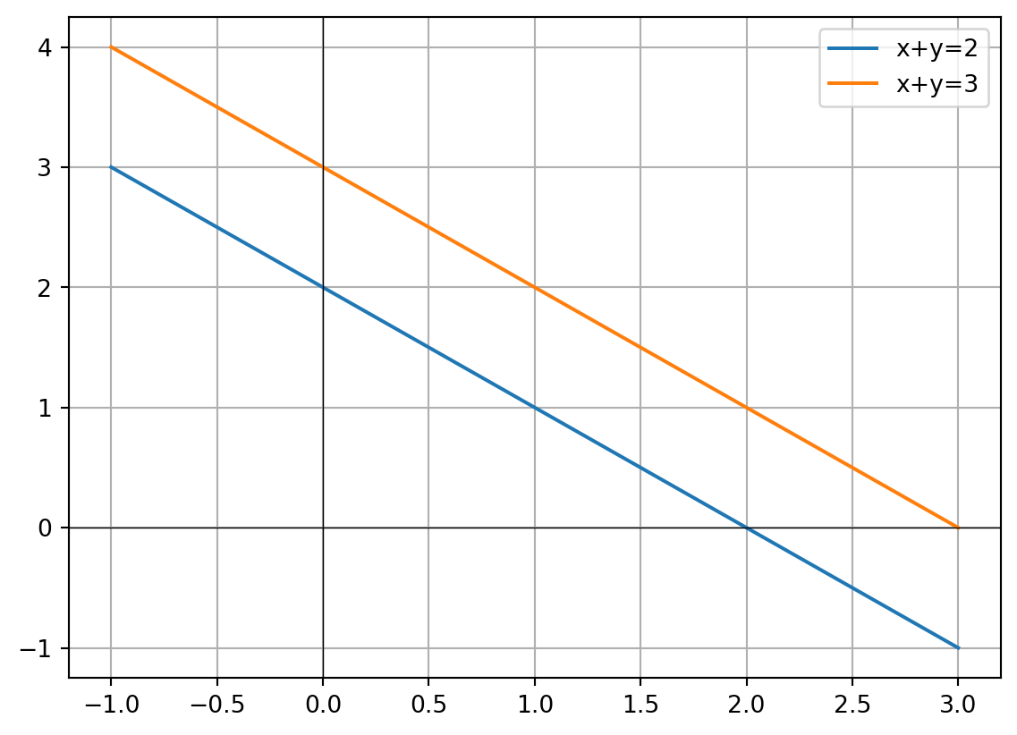
The two lines are parallel → no solution.

Detecting inconsistency automatically

We can scan the RREF for a row of the form \([0, 0, …, c]\) with \(c \neq 0\).

def is_inconsistent(M):
= M.rref()
for row in rref_matrix.tolist():
if all(v == 0 for v in row[:-1]) and row[-1] != 0:
return True
return False

print("System 1 inconsistent?", is_inconsistent(M))
print("System 2 inconsistent?", is_inconsistent(M2))

System 1 inconsistent? True
System 2 inconsistent? False

Try It Yourself

Test the system:

\[
x + 2y = 4, \quad 2x + 4y = 10
\]

Write the augmented matrix and check if it’s inconsistent.
Build a random 2×3 augmented matrix with integer entries. Use is_inconsistent to check.
Plot two linear equations in 2D. Adjust constants to see when they intersect (consistent) vs when they are parallel (inconsistent).

The Takeaway

A system is inconsistent if RREF contains a row like \([0,0,…,c]\) with \(c \neq 0\).
Geometrically, this means the equations describe parallel lines (2D), parallel planes (3D), or higher-dimensional contradictions.
Recognizing inconsistency quickly saves time and avoids chasing impossible solutions.

27. Gaussian Elimination by Hand (A Disciplined Procedure)

Gaussian elimination is the systematic way to solve linear systems using row operations. It transforms the augmented matrix into row-echelon form (REF) and then uses back substitution to find solutions. In this lab, we’ll walk step by step through the process.

Set Up Your Lab

import numpy as np
from sympy import Matrix

Step-by-Step Code Walkthrough

Example system

\[
\begin{cases}
x + y + z = 6 \\
2x + 3y + z = 14 \\
x + 2y + 3z = 14
\end{cases}
\]

= np.array([
1, 1, 1, 6],
2, 3, 1, 14],
1, 2, 3, 14]
=float)

print("Initial augmented matrix:\n", A)

Initial augmented matrix:
 [[ 1.  1.  1.  6.]
 [ 2.  3.  1. 14.]
 [ 1.  2.  3. 14.]]

Step 1: Get a pivot in the first column

Make the pivot at (0,0) into 1 (it already is). Now eliminate below it.

1] = A[1] - 2*A[0]   # Row2 → Row2 - 2*Row1
2] = A[2] - A[0]     # Row3 → Row3 - Row1
print("After eliminating first column:\n", A)

After eliminating first column:
 [[ 1.  1.  1.  6.]
 [ 0.  1. -1.  2.]
 [ 0.  1.  2.  8.]]

Step 2: Pivot in the second column

Make the pivot in row 1, col 1 equal to 1.

1] = A[1] / A[1,1]
print("After scaling second row:\n", A)

After scaling second row:
 [[ 1.  1.  1.  6.]
 [ 0.  1. -1.  2.]
 [ 0.  1.  2.  8.]]

Now eliminate below:

2] = A[2] - A[2,1]*A[1]
print("After eliminating second column:\n", A)

After eliminating second column:
 [[ 1.  1.  1.  6.]
 [ 0.  1. -1.  2.]
 [ 0.  0.  3.  6.]]

Step 3: Pivot in the third column

Make the bottom-right entry into 1.

2] = A[2] / A[2,2]
print("After scaling third row:\n", A)

After scaling third row:
 [[ 1.  1.  1.  6.]
 [ 0.  1. -1.  2.]
 [ 0.  0.  1.  2.]]

At this point, the matrix is in row-echelon form (REF).

Back substitution

Now solve from the bottom up:

= A[2,3]
= A[1,3] - A[1,2]*z
= A[0,3] - A[0,1]*y - A[0,2]*z

print(f"Solution: x={x}, y={y}, z={z}")

Solution: x=0.0, y=4.0, z=2.0

Verification

= np.array([
1,1,1],
2,3,1],
1,2,3]
=float)
= np.array([6,14,14], dtype=float)

print("Check with np.linalg.solve:", np.linalg.solve(coeff,const))

Check with np.linalg.solve: [0. 4. 2.]

The results match.

Try It Yourself

Solve:

\[
2x + y = 5, \quad 4x – 6y = -2
\]

using Gaussian elimination manually in code.
Create a random 3×4 augmented matrix and reduce it step by step, printing after each row operation.
Compare your manual elimination to SymPy’s RREF with Matrix.rref().

The Takeaway

Gaussian elimination is a disciplined sequence of row operations.
It reduces the matrix to row-echelon form, from which back substitution is straightforward.
This method is the backbone of solving systems by hand and underlies many numerical algorithms.

28. Back Substitution and Solution Sets (Finishing Cleanly)

Once Gaussian elimination reduces a system to row-echelon form (REF), the final step is back substitution. This means solving variables starting from the last equation and working upward. In this lab, we’ll practice both unique and infinite solution cases.

Set Up Your Lab

import numpy as np
from sympy import Matrix

Step-by-Step Code Walkthrough

Unique solution example

System:

\[
x + y + z = 6, \quad 2y + 5z = -4, \quad z = 3
\]

Row-echelon form looks like:

\[
\begin{bmatrix}
1 & 1 & 1 & 6 \\
0 & 2 & 5 & -4 \\
0 & 0 & 1 & 3
\end{bmatrix}
\]

Solve bottom-up:

= 3
= (-4 - 5*z)/2
= 6 - y - z
print(f"Solution: x={x}, y={y}, z={z}")

Solution: x=12.5, y=-9.5, z=3

Infinite solution example

System:

\[
x + y + z = 2, \quad 2x + 2y + 2z = 4
\]

After elimination:

\[
\begin{bmatrix}
1 & 1 & 1 & 2 \\
0 & 0 & 0 & 0
\end{bmatrix}
\]

This means:

Equation: \(x + y + z = 2\).
Free variables: choose \(y\) and \(z\).

Let \(y = s, z = t\). Then:

\[
x = 2 – s – t
\]

So the solution set is:

from sympy import symbols
= symbols('s t')
= 2 - s - t
= s
= t
print("General solution:")
print("x =", x, ", y =", y, ", z =", z)

General solution:
x = -s - t + 2 , y = s , z = t

Consistency check with RREF

We can use SymPy to confirm solution sets:

= Matrix([
1,1,1,2],
2,2,2,4]


print("RREF form:\n", M.rref()[0])

RREF form:
 Matrix([[1, 1, 1, 2], [0, 0, 0, 0]])

The second row disappears, showing infinite solutions.

Encoding solution sets

General solutions are often written in parametric vector form.

For the infinite solution above:

\[
(x,y,z) = (2,0,0) + s(-1,1,0) + t(-1,0,1)
\]

This shows the solution space is a plane in \(\mathbb{R}^3\).

Try It Yourself

Solve:

\[
x + 2y = 5, \quad y = 1
\]

Do back substitution by hand and check with NumPy.
Take the system:

\[
x + y + z = 1, \quad 2x + 2y + 2z = 2
\]

Write its solution set in parametric form.
Use Matrix.rref() on a 3×4 random augmented matrix. Identify pivot and free variables, then describe the solution set.

The Takeaway

Back substitution is the cleanup step after Gaussian elimination.
It reveals whether the system has a unique solution or infinitely many.
Solutions can be expressed explicitly (unique case) or parametrically (infinite case).

29. Rank and Its First Meaning (Pivots as Information)

The rank of a matrix tells us how much independent information it contains. Rank is one of the most important concepts in linear algebra because it connects to pivots, independence, dimension, and the number of solutions to a system.

Set Up Your Lab

import numpy as np
from sympy import Matrix

Step-by-Step Code Walkthrough

Rank definition The rank is the number of pivots (leading ones) in the row-echelon form of a matrix.

Example:

= Matrix([
1, 2, 3],
2, 4, 6],
1, 1, 1]


print("RREF:\n", A.rref()[0])
print("Rank of A:", A.rank())

RREF:
 Matrix([[1, 0, -1], [0, 1, 2], [0, 0, 0]])
Rank of A: 2

The second row is a multiple of the first, so the rank is less than 3.
Only two independent rows → rank = 2.

Rank and solutions to \(A·x = b\)

Consider:

\[
\begin{cases}
x + y + z = 3 \\
2x + 2y + 2z = 6 \\
x – y = 0
\end{cases}
\]

= Matrix([
1, 1, 1, 3],
2, 2, 2, 6],
1, -1, 0, 0]


print("RREF:\n", M.rref()[0])
print("Rank of coefficient matrix:", M[:, :-1].rank())
print("Rank of augmented matrix:", M.rank())

RREF:
 Matrix([[1, 0, 1/2, 3/2], [0, 1, 1/2, 3/2], [0, 0, 0, 0]])
Rank of coefficient matrix: 2
Rank of augmented matrix: 2

If rank(A) = rank([A|b]) = number of variables → unique solution.
If rank(A) = rank([A|b]) < number of variables → infinite solutions.
If rank(A) < rank([A|b]) → no solution.

NumPy comparison

= np.array([
1, 2, 3],
2, 4, 6],
1, 1, 1]
=float)

print("Rank with NumPy:", np.linalg.matrix_rank(A))

Rank with NumPy: 2

Rank as “dimension of information”

The rank equals:

The number of independent rows.
The number of independent columns.
The dimension of the column space.

= Matrix([
1,2],
2,4],
3,6]


print("Rank of B:", B.rank())

Rank of B: 1

All columns are multiples → only one independent direction → rank = 1.

Try It Yourself

Compute the rank of:

\[
\begin{bmatrix}
1 & 2 & 3 \\
2 & 4 & 6 \\
3 & 6 & 9
\end{bmatrix}
\]

What do you expect?
Create a random 4×4 matrix with np.random.randint. Compute its rank with both SymPy and NumPy.
Test solution consistency using rank: build a system where rank(A) ≠ rank([A|b]) and show it has no solution.

The Takeaway

Rank = number of pivots = dimension of independent information.
Rank reveals whether a system has no solution, one solution, or infinitely many.
Rank connects algebra (pivots) with geometry (dimension of subspaces).

30. LU Factorization (Elimination Captured as L and U)

Gaussian elimination can be recorded in a neat factorization:

\[
A = LU
\]

where \(L\) is a lower triangular matrix (recording the multipliers we used) and \(U\) is an upper triangular matrix (the result of elimination). This is called LU factorization. It’s a powerful tool for solving systems efficiently.

Set Up Your Lab

import numpy as np
from scipy.linalg import lu

Step-by-Step Code Walkthrough

Example matrix

= np.array([
2, 3, 1],
4, 7, 7],
6, 18, 22]
=float)

print("Matrix A:\n", A)

Matrix A:
 [[ 2.  3.  1.]
 [ 4.  7.  7.]
 [ 6. 18. 22.]]

LU decomposition with SciPy

= lu(A)

print("Permutation matrix P:\n", P)
print("Lower triangular L:\n", L)
print("Upper triangular U:\n", U)

Permutation matrix P:
 [[0. 0. 1.]
 [0. 1. 0.]
 [1. 0. 0.]]
Lower triangular L:
 [[1.         0.         0.        ]
 [0.66666667 1.         0.        ]
 [0.33333333 0.6        1.        ]]
Upper triangular U:
 [[ 6.         18.         22.        ]
 [ 0.         -5.         -7.66666667]
 [ 0.          0.         -1.73333333]]

Here, \(P\) handles row swaps (partial pivoting), \(L\) is lower triangular, and \(U\) is upper triangular.

Verifying the factorization

= P @ L @ U
print("Does P·L·U equal A?\n", np.allclose(reconstructed, A))

Does P·L·U equal A?
 True

Solving a system with LU

Suppose we want to solve \(Ax = b\). Instead of working directly with \(A\), we solve in two steps:

Solve \(Ly = Pb\) (forward substitution).
Solve \(Ux = y\) (back substitution).

= np.array([1, 2, 3], dtype=float)

# Step 1: Pb
= P @ b

# Step 2: forward substitution Ly = Pb
= np.linalg.solve(L, Pb)

# Step 3: back substitution Ux = y
= np.linalg.solve(U, y)

print("Solution x:", x)

Solution x: [ 0.5 -0.  -0. ]

Efficiency advantage

If we have to solve many systems with the same \(A\) but different \(b\), we only compute \(LU\) once, then reuse it. This saves a lot of computation.

NumPy’s built-in rank-revealing factorization

While NumPy doesn’t have lu directly, it works seamlessly with SciPy. For large matrices, LU decomposition is the backbone of solvers like np.linalg.solve.

Try It Yourself

Compute LU decomposition for

\[
A = \begin{bmatrix} 1 & 2 & 0 \\ 3 & 4 & 4 \\ 5 & 6 & 3 \end{bmatrix}
\]

Verify \(P·L·U = A\).
Solve \(Ax = b\) with

\[
b = [3,7,8]
\]

using LU factorization.
Compare solving with LU factorization vs directly using np.linalg.solve(A,b). Are the answers the same?

The Takeaway

LU factorization captures Gaussian elimination in matrix form: \(A = P·L·U\).
It allows fast repeated solving of systems with different right-hand sides.
LU decomposition is a core technique in numerical linear algebra and the basis of many solvers.

Chapter 4. Vector Spaces and Subspaces

31. Axioms of Vector Spaces (What “Space” Really Means)

Vector spaces generalize what we’ve been doing with vectors and matrices. Instead of just \(\mathbb{R}^n\), a vector space is any collection of objects (vectors) where addition and scalar multiplication follow specific axioms (rules). In this lab, we’ll explore these axioms concretely with Python.

Set Up Your Lab

import numpy as np

Step-by-Step Code Walkthrough

Vector space example: \(\mathbb{R}^2\)

Let’s check two rules (axioms): closure under addition and scalar multiplication.

= np.array([1, 2])
= np.array([3, -1])

# Closure under addition
print("u + v =", u + v)

# Closure under scalar multiplication
= 5
print("k * u =", k * u)

u + v = [4 1]
k * u = [ 5 10]

Both results are still in \(\mathbb{R}^2\).

Zero vector and additive inverses

Every vector space must contain a zero vector, and every vector must have an additive inverse.

= np.array([0, 0])
= -u
print("Zero vector:", zero)
print("u + (-u) =", u + inverse_u)

Zero vector: [0 0]
u + (-u) = [0 0]

Distributive and associative properties

Check:

\(a(u+v) = au + av\)
\((a+b)u = au + bu\)

= 2, 3

= a * (u + v)
= a*u + a*v
print("a(u+v) =", lhs1, ", au+av =", rhs1)

= (a+b) * u
= a*u + b*u
print("(a+b)u =", lhs2, ", au+bu =", rhs2)

a(u+v) = [8 2] , au+av = [8 2]
(a+b)u = [ 5 10] , au+bu = [ 5 10]

Both equalities hold → distributive laws confirmed.

A set that fails to be a vector space

Consider only positive numbers with normal addition and scalar multiplication.

= [1, 2, 3]
try:
print("Closure under negatives?", -1 * np.array(positive_numbers))
except Exception as e:
print("Error:", e)

Closure under negatives? [-1 -2 -3]

Negative results leave the set → not a vector space.

Python helper to check axioms

We can quickly check if a set of vectors is closed under addition and scalar multiplication.

def check_closure(vectors, scalars):
for v in vectors:
for u in vectors:
if not any(np.array_equal(v+u, w) for w in vectors):
return False
for k in scalars:
if not any(np.array_equal(k*v, w) for w in vectors):
return False
return True

= [np.array([0,0]), np.array([1,0]), np.array([0,1]), np.array([1,1])]
= [0,1,-1]
print("Closed under addition and scalar multiplication?", check_closure(vectors, scalars))

Closed under addition and scalar multiplication? False

This small set is closed → it forms a vector space (a subspace of \(\mathbb{R}^2\)).

Try It Yourself

Verify that \(\mathbb{R}^3\) satisfies the vector space axioms using random vectors.
Test whether the set of all 2×2 matrices forms a vector space under normal addition and scalar multiplication.
Find an example of a set that fails closure (e.g., integers under division).

The Takeaway

A vector space is any set where addition and scalar multiplication satisfy 10 standard axioms.
These rules ensure consistent algebraic behavior.
Many objects beyond arrows in \(\mathbb{R}^n\) (like polynomials or matrices) are vector spaces too.

32. Subspaces, Column Space, and Null Space (Where Solutions Live)

A subspace is a smaller vector space sitting inside a bigger one. For matrices, two subspaces show up all the time:

Column space: all combinations of the matrix’s columns (possible outputs of \(Ax\)).
Null space: all vectors \(x\) such that \(Ax = 0\) (inputs that vanish).

This lab explores both in Python.

Set Up Your Lab

import numpy as np
from sympy import Matrix

Step-by-Step Code Walkthrough

Column space basics

Take:

\[
A = \begin{bmatrix} 1 & 2 \\ 2 & 4 \\ 3 & 6 \end{bmatrix}
\]

= Matrix([
1,2],
2,4],
3,6]


print("Matrix A:\n", A)
print("Column space basis:\n", A.columnspace())
print("Rank (dimension of column space):", A.rank())

Matrix A:
 Matrix([[1, 2], [2, 4], [3, 6]])
Column space basis:
 [Matrix([
[1],
[2],
[3]])]
Rank (dimension of column space): 1

The second column is a multiple of the first → column space has dimension 1.
All outputs of \(Ax\) lie on a line in \(\mathbb{R}^3\).

Null space basics

print("Null space basis:\n", A.nullspace())

Null space basis:
 [Matrix([
[-2],
[ 1]])]

The null space contains all \(x\) where \(Ax=0\). Here, the null space is 1-dimensional (vectors like \([-2,1]\)).

A full-rank example

= Matrix([
1,0,0],
0,1,0],
0,0,1]


print("Column space basis:\n", B.columnspace())
print("Null space basis:\n", B.nullspace())

Column space basis:
 [Matrix([
[1],
[0],
[0]]), Matrix([
[0],
[1],
[0]]), Matrix([
[0],
[0],
[1]])]
Null space basis:
 []

Column space = all of \(\mathbb{R}^3\).
Null space = only the zero vector.

Geometry link

For \(A\) (rank 1, 2 columns):

Column space: line in \(\mathbb{R}^3\).
Null space: line in \(\mathbb{R}^2\).

Together they explain the system \(Ax = b\):

If \(b\) is outside the column space, no solution exists.
If \(b\) is inside, solutions differ by a vector in the null space.

Quick NumPy version

NumPy doesn’t directly give null space, but we can compute it with SVD.

from numpy.linalg import svd

= np.array([[1,2],[2,4],[3,6]], dtype=float)
= svd(A)

= 1e-10
= (S <= tol)
= Vt.T[:, null_mask]
print("Null space (via SVD):\n", null_space)

Null space (via SVD):
 [[-0.89442719]
 [ 0.4472136 ]]

Try It Yourself

Find the column space and null space of

\[
\begin{bmatrix} 1 & 1 \\ 0 & 1 \\ 0 & 0 \end{bmatrix}
\]

How many dimensions does each have?
Generate a random 3×3 matrix. Compute its rank, column space, and null space.
Solve \(Ax = b\) with

\[
A = \begin{bmatrix} 1 & 2 \\ 2 & 4 \\ 3 & 6 \end{bmatrix}, \quad b = \begin{bmatrix} 1 \\ 2 \\ 3 \end{bmatrix}
\]

and describe why it has infinitely many solutions.

The Takeaway

The column space = all possible outputs of a matrix.
The null space = all inputs that map to zero.
These subspaces give the complete picture of what a matrix does.

33. Span and Generating Sets (Coverage of a Space)

The span of a set of vectors is all the linear combinations you can make from them. If a set of vectors can “cover” a whole space, we call it a generating set. This lab shows how to compute and visualize spans.

Set Up Your Lab

import numpy as np
from sympy import Matrix
import matplotlib.pyplot as plt

Step-by-Step Code Walkthrough

Span in \(\mathbb{R}^2\)

Two vectors that aren’t multiples span the whole plane.

= np.array([1, 0])
= np.array([0, 1])

= Matrix.hstack(Matrix(u), Matrix(v))
print("Rank:", M.rank())

Rank: 2

Rank = 2 → the span of \(\{u,v\}\) is all of \(\mathbb{R}^2\).

Dependent vectors (smaller span)

= np.array([1, 2])
= np.array([2, 4])

= Matrix.hstack(Matrix(u), Matrix(v))
print("Rank:", M.rank())

Rank: 1

Rank = 1 → these vectors only span a line.

Visualizing a span

Let’s see what the span of two vectors looks like.

= np.array([1, 2])
= np.array([2, 1])

= np.linspace(-2, 2, 11)
= []
for a in coeffs:
for b in coeffs:
*u + b*v)
= np.array(points)

0], points[:,1], s=10)
0,color='black',linewidth=0.5)
0,color='black',linewidth=0.5)
"Span of {u,v}")

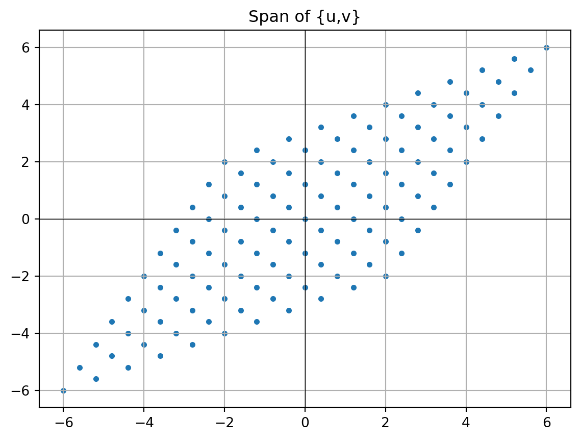
You’ll see a filled grid – the entire plane, because the two vectors are independent.

Generating set of a space

For \(\mathbb{R}^3\):

= [Matrix([1,0,0]), Matrix([0,1,0]), Matrix([0,0,1])]
= Matrix.hstack(*basis)
print("Rank:", M.rank())

Rank: 3

Rank = 3 → this set spans the whole space.

Testing if a vector is in the span

Example: Is \([3,5]\) in the span of \([1,2]\) and \([2,1]\)?

= Matrix([1,2])
= Matrix([2,1])
= Matrix([3,5])

= Matrix.hstack(u,v)
= M.gauss_jordan_solve(target)
print("Coefficients (a,b):", solution)

Coefficients (a,b): (Matrix([
[7/3],
[1/3]]), Matrix(0, 1, []))

If a solution exists, the target is in the span.

Try It Yourself

Test if \([4,6]\) is in the span of \([1,2]\).
Visualize the span of \([1,0,0]\) and \([0,1,0]\) in \(\mathbb{R}^3\). What does it look like?
Create a random 3×3 matrix. Use rank() to check if its columns span \(\mathbb{R}^3\).

The Takeaway

Span = all linear combinations of a set of vectors.
Independent vectors span bigger spaces; dependent ones collapse to smaller spaces.
Generating sets are the foundation of bases and coordinate systems.

34. Linear Independence and Dependence (No Redundancy vs. Redundancy)

A set of vectors is linearly independent if none of them can be written as a combination of the others. If at least one can, the set is dependent. This distinction tells us whether a set of vectors has redundancy.

Set Up Your Lab

import numpy as np
from sympy import Matrix

Step-by-Step Code Walkthrough

Independent vectors example

= Matrix([1, 0, 0])
= Matrix([0, 1, 0])
= Matrix([0, 0, 1])

= Matrix.hstack(v1, v2, v3)
print("Rank:", M.rank(), " Number of vectors:", M.shape[1])

Rank: 3  Number of vectors: 3

Rank = 3, number of vectors = 3 → all independent.

Dependent vectors example

= Matrix([1, 2, 3])
= Matrix([2, 4, 6])
= Matrix([3, 6, 9])

= Matrix.hstack(v1, v2, v3)
print("Rank:", M.rank(), " Number of vectors:", M.shape[1])

Rank: 1  Number of vectors: 3

Rank = 1, number of vectors = 3 → they’re dependent (multiples of each other).

Checking dependence automatically

A quick test: if rank < number of vectors → dependent.

def check_independence(vectors):
= Matrix.hstack(*vectors)
return M.rank() == M.shape[1]

print("Independent?", check_independence([Matrix([1,0]), Matrix([0,1])]))
print("Independent?", check_independence([Matrix([1,2]), Matrix([2,4])]))

Independent? True
Independent? False

Solving for dependence relation

If vectors are dependent, we can find coefficients \(c_1, c_2, …\) such that

\[
c_1 v_1 + c_2 v_2 + … + c_k v_k = 0
\]

with some \(c_i \neq 0\).

= Matrix.hstack(Matrix([1,2]), Matrix([2,4]))
= M.nullspace()
print("Dependence relation (coefficients):", null_space)

Dependence relation (coefficients): [Matrix([
[-2],
[ 1]])]

This shows the exact linear relation.

Random example

0)
= Matrix(np.random.randint(-3, 4, (3,3)))
print("Random matrix:\n", R)
print("Rank:", R.rank())

Random matrix:
 Matrix([[1, 2, -3], [0, 0, 0], [-2, 0, 2]])
Rank: 2

Depending on the rank, the columns may be independent (rank = 3) or dependent (rank < 3).

Try It Yourself

Test if \([1,1,0], [0,1,1], [1,2,1]\) are independent.
Generate 4 random vectors in \(\mathbb{R}^3\). Can they ever be independent? Why or why not?
Find the dependence relation for \([2,4], [3,6]\).

The Takeaway

Independent set: no redundancy, each vector adds a new direction.
Dependent set: at least one vector is unnecessary (it lies in the span of others).
Independence is the key to defining basis and dimension.

35. Basis and Coordinates (Naming Every Vector Uniquely)

A basis is a set of independent vectors that span a space. It’s like choosing a coordinate system: every vector in the space can be expressed uniquely as a combination of basis vectors. In this lab, we’ll see how to find bases and compute coordinates relative to them.

Set Up Your Lab

import numpy as np
from sympy import Matrix

Step-by-Step Code Walkthrough

Standard basis in \(\mathbb{R}^3\)

= Matrix([1,0,0])
= Matrix([0,1,0])
= Matrix([0,0,1])

= Matrix.hstack(e1, e2, e3)
print("Rank:", M.rank())

Rank: 3

These three independent vectors form the standard basis of \(\mathbb{R}^3\). Any vector like \([2,5,-1]\) can be expressed as

\[
2e_1 + 5e_2 – 1e_3
\]

Finding a basis from dependent vectors

= Matrix([1,2,3])
= Matrix([2,4,6])
= Matrix([1,0,1])

= Matrix.hstack(v1,v2,v3)
print("Column space basis:", M.columnspace())

Column space basis: [Matrix([
[1],
[2],
[3]]), Matrix([
[1],
[0],
[1]])]

SymPy extracts independent columns automatically. This gives a basis for the column space.

Coordinates relative to a basis

Suppose basis = \(\{ [1,0], [1,1] \}\). Express vector \([3,5]\) in this basis.

= Matrix.hstack(Matrix([1,0]), Matrix([1,1]))
= Matrix([3,5])

= B.solve_least_squares(target)
print("Coordinates in basis B:", coords)

Coordinates in basis B: Matrix([[-2], [5]])

So \([3,5] = 3·[1,0] + 2·[1,1]\).

Basis change

If we switch to a different basis, coordinates change but the vector stays the same.

= Matrix.hstack(Matrix([2,1]), Matrix([1,2]))
= new_basis.solve_least_squares(target)
print("Coordinates in new basis:", coords_new)

Coordinates in new basis: Matrix([[1/3], [7/3]])

Random example

Generate 3 random vectors in \(\mathbb{R}^3\). Check if they form a basis.

1)
= Matrix(np.random.randint(-3,4,(3,3)))
print("Random matrix:\n", R)
print("Rank:", R.rank())

Random matrix:
 Matrix([[2, 0, 1], [-3, -2, 0], [2, -3, -3]])
Rank: 3

If rank = 3 → basis for \(\mathbb{R}^3\). Otherwise, only span a subspace.

Try It Yourself

Check if \([1,2], [3,4]\) form a basis of \(\mathbb{R}^2\).
Express vector \([7,5]\) in that basis.
Create 4 random vectors in \(\mathbb{R}^3\). Find a basis for their span.

The Takeaway

A basis = minimal set of vectors that span a space.
Every vector has a unique coordinate representation in a given basis.
Changing bases changes the coordinates, not the vector itself.

36. Dimension (How Many Directions)

The dimension of a vector space is the number of independent directions it has. Formally, it’s the number of vectors in any basis of the space. Dimension tells us the “size” of a space in terms of degrees of freedom.

Set Up Your Lab

import numpy as np
from sympy import Matrix

Step-by-Step Code Walkthrough

Dimension of \(\mathbb{R}^n\)

The dimension of \(\mathbb{R}^n\) is \(n\).

= 4
= [Matrix.eye(n)[:,i] for i in range(n)]
print("Basis for R^4:", basis)
print("Dimension of R^4:", len(basis))

Basis for R^4: [Matrix([
[1],
[0],
[0],
[0]]), Matrix([
[0],
[1],
[0],
[0]]), Matrix([
[0],
[0],
[1],
[0]]), Matrix([
[0],
[0],
[0],
[1]])]
Dimension of R^4: 4

Each standard unit vector adds one independent direction → dimension = 4.

Dimension via rank

The rank of a matrix equals the dimension of its column space.

= Matrix([
1,2,3],
2,4,6],
1,0,1]


print("Rank (dimension of column space):", A.rank())

Rank (dimension of column space): 2

Here, rank = 2 → the column space is a 2D plane inside \(\mathbb{R}^3\).

Null space dimension

The null space dimension is given by:

\[
\text{dim(Null(A))} = \#\text{variables} – \text{rank(A)}
\]

print("Null space basis:", A.nullspace())
print("Dimension of null space:", len(A.nullspace()))

Null space basis: [Matrix([
[-1],
[-1],
[ 1]])]
Dimension of null space: 1

This is the number of free variables in a solution.

Dimension in practice

A line through the origin in \(\mathbb{R}^3\) has dimension 1.
A plane through the origin has dimension 2.
The whole \(\mathbb{R}^3\) has dimension 3.

Example:

= Matrix([1,2,3])
= Matrix([2,4,6])
= Matrix.hstack(v1,v2)
print("Dimension of span:", span.rank())

Dimension of span: 1

Result = 1 → they only generate a line.

Random example

2)
= Matrix(np.random.randint(-3,4,(4,4)))
print("Random 4x4 matrix:\n", R)
print("Column space dimension:", R.rank())

Random 4x4 matrix:
 Matrix([[-3, 2, -3, 3], [0, -1, 0, -3], [-1, -2, 0, 2], [-1, 1, 1, 1]])
Column space dimension: 4

Rank may be 4 (full space) or smaller (collapsed).

Try It Yourself

Find the dimension of the column space of

\[
\begin{bmatrix}
1 & 1 & 1 \\
0 & 1 & 1 \\
0 & 0 & 0
\end{bmatrix}
\]
Compute the dimension of the null space of a 3×3 singular matrix.
Generate a 5×3 random matrix and compute its column space dimension.

The Takeaway

Dimension = number of independent directions.
Found by counting basis vectors (or rank).
Dimensions describe lines (1D), planes (2D), and higher subspaces inside larger spaces.

37. Rank–Nullity Theorem (Dimensions That Add Up)

The rank–nullity theorem ties together the dimension of the column space and the null space of a matrix. It says:

\[
\text{rank}(A) + \text{nullity}(A) = \text{number of columns of } A
\]

This is a powerful consistency check in linear algebra.

Set Up Your Lab

import numpy as np
from sympy import Matrix

Step-by-Step Code Walkthrough

Simple 3×3 example

= Matrix([
1, 2, 3],
2, 4, 6],
1, 0, 1]


= A.rank()
= len(A.nullspace())
print("Rank:", rank)
print("Nullity:", nullity)
print("Rank + Nullity =", rank + nullity)
print("Number of columns =", A.shape[1])

Rank: 2
Nullity: 1
Rank + Nullity = 3
Number of columns = 3

You should see that rank + nullity = 3, the number of columns.

Full-rank case

= Matrix([
1,0,0],
0,1,0],
0,0,1]


print("Rank:", B.rank())
print("Nullity:", len(B.nullspace()))

Rank: 3
Nullity: 0

Rank = 3 (all independent).
Nullity = 0 (only zero solution to \(Bx=0\)).
Rank + Nullity = 3 columns.

Wide matrix (more columns than rows)

= Matrix([
1,2,3,4],
0,1,1,2],
0,0,0,0]


= C.rank()
= len(C.nullspace())
print("Rank:", rank, " Nullity:", nullity, " Columns:", C.shape[1])

Rank: 2  Nullity: 2  Columns: 4

Here, nullity > 0 because there are more variables than independent equations.

Verifying with random matrices

3)
= Matrix(np.random.randint(-3,4,(4,5)))
print("Random 4x5 matrix:\n", R)
print("Rank + Nullity =", R.rank() + len(R.nullspace()))
print("Number of columns =", R.shape[1])

Random 4x5 matrix:
 Matrix([[-1, -3, -2, 0, -3], [-3, -3, 2, 2, 0], [-1, 0, -2, -2, -1], [2, 3, -3, 1, 1]])
Rank + Nullity = 5
Number of columns = 5

Always consistent: rank + nullity = number of columns.

Geometric interpretation

For an \(m \times n\) matrix:

Rank(A) = dimension of outputs (column space).
Nullity(A) = dimension of hidden directions that collapse to 0.
Together, they use up all the “input dimensions” (n).

Try It Yourself

Compute rank and nullity of

\[
\begin{bmatrix}
1 & 1 & 1 \\
0 & 1 & 1
\end{bmatrix}
\]

Check the theorem.
Create a 2×4 random integer matrix. Confirm that rank + nullity = 4.
Explain why a tall full-rank \(5 \times 3\) matrix must have nullity = 0.

The Takeaway

Rank + Nullity = number of columns (always true).
Rank measures independent outputs; nullity measures hidden freedom.
This theorem connects solutions of \(Ax=0\) with the structure of \(A\).

38. Coordinates Relative to a Basis (Changing the “Ruler”)

Once we choose a basis, every vector can be described with coordinates relative to that basis. This is like changing the “ruler” we use to measure vectors. In this lab, we’ll practice computing coordinates in different bases.

Set Up Your Lab

import numpy as np
from sympy import Matrix

Step-by-Step Code Walkthrough

Standard basis coordinates

Vector \(v = [4,5]\) in \(\mathbb{R}^2\):

= Matrix([4,5])
= Matrix([1,0])
= Matrix([0,1])

= Matrix.hstack(e1,e2)
= B.solve_least_squares(v)
print("Coordinates in standard basis:", coords)

Coordinates in standard basis: Matrix([[4], [5]])

Result is just \([4,5]\). Easy – the standard basis matches the components directly.

Non-standard basis

Suppose basis = \(\{ [1,1], [1,-1] \}\). Express \(v = [4,5]\) in this basis.

= Matrix.hstack(Matrix([1,1]), Matrix([1,-1]))
= B2.solve_least_squares(v)
print("Coordinates in new basis:", coords2)

Coordinates in new basis: Matrix([[9/2], [-1/2]])

Now \(v\) has different coordinates.

Changing coordinates back

To reconstruct the vector from coordinates:

= B2 * coords2
print("Reconstructed vector:", reconstructed)

Reconstructed vector: Matrix([[4], [5]])

It matches the original \([4,5]\).

Random basis in \(\mathbb{R}^3\)

= Matrix.hstack(
1,0,1]),
0,1,1]),
1,1,0])

= Matrix([2,3,4])

= basis.solve_least_squares(v)
print("Coordinates of v in random basis:", coords)

Coordinates of v in random basis: Matrix([[3/2], [5/2], [1/2]])

Any independent set of 3 vectors in \(\mathbb{R}^3\) works as a basis.

Visualization in 2D

Let’s compare coordinates in two bases.

import matplotlib.pyplot as plt

= np.array([4,5])
= np.array([1,1])
= np.array([1,-1])

0,0,v[0],v[1],angles='xy',scale_units='xy',scale=1,color='blue',label='v')
0,0,b1[0],b1[1],angles='xy',scale_units='xy',scale=1,color='red',label='basis1')
0,0,b2[0],b2[1],angles='xy',scale_units='xy',scale=1,color='green',label='basis2')

-1,6)
-6,6)

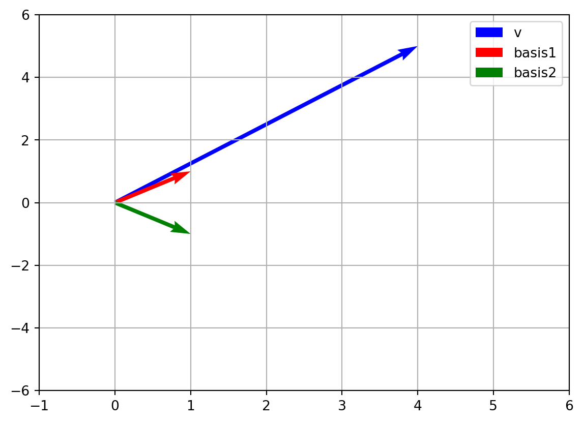
Even though the basis vectors look different, they span the same space, and \(v\) can be expressed in terms of them.

Try It Yourself

Express \([7,3]\) in the basis \(\{[2,0], [0,3]\}\).
Pick three independent random vectors in \(\mathbb{R}^3\). Write down the coordinates of \([1,2,3]\) in that basis.
Verify that reconstructing always gives the original vector.

The Takeaway

A basis provides a coordinate system for vectors.
Coordinates depend on the basis, but the underlying vector doesn’t change.
Changing the basis is like changing the “ruler” you measure vectors with.

39. Change-of-Basis Matrices (Moving Between Coordinate Systems)

When we switch from one basis to another, we need a change-of-basis matrix. This matrix acts like a translator: it converts coordinates in one system to coordinates in another.

Set Up Your Lab

import numpy as np
from sympy import Matrix

Step-by-Step Code Walkthrough

Two bases in \(\mathbb{R}^2\)

Let’s define:

Basis \(B = \{ [1,0], [0,1] \}\) (standard basis).
Basis \(C = \{ [1,1], [1,-1] \}\).

= Matrix.hstack(Matrix([1,0]), Matrix([0,1]))
= Matrix.hstack(Matrix([1,1]), Matrix([1,-1]))

Change-of-basis matrix

The matrix that converts C-coordinates → standard coordinates is just \(C\).

print("C (basis matrix):\n", C)

C (basis matrix):
 Matrix([[1, 1], [1, -1]])

To go the other way (standard → C), we compute the inverse of \(C\).

= C.inv()
print("C inverse:\n", C_inv)

C inverse:
 Matrix([[1/2, 1/2], [1/2, -1/2]])

Converting coordinates

Vector \(v = [4,5]\).

In standard basis:

= Matrix([4,5])
= v
print("Coordinates in standard basis:", coords_in_standard)

Coordinates in standard basis: Matrix([[4], [5]])

In basis \(C\):

= C_inv * v
print("Coordinates in C basis:", coords_in_C)

Coordinates in C basis: Matrix([[9/2], [-1/2]])

Convert back:

= C * coords_in_C
print("Reconstructed vector:", reconstructed)

Reconstructed vector: Matrix([[4], [5]])

The reconstruction matches the original vector.

General formula

If \(P\) is the change-of-basis matrix from basis \(B\) to basis \(C\):

\[
[v]_C = P^{-1}[v]_B
\]

\[
[v]_B = P[v]_C
\]

Here, \(P\) is the matrix of new basis vectors written in terms of the old basis.

Random 3D example

= Matrix.eye(3)  # standard basis
= Matrix.hstack(
1,0,1]),
0,1,1]),
1,1,0])


= Matrix([2,3,4])

= C.inv()
= C_inv * v
print("Coordinates in new basis C:", coords_in_C)

print("Back to standard:", C * coords_in_C)

Coordinates in new basis C: Matrix([[3/2], [5/2], [1/2]])
Back to standard: Matrix([[2], [3], [4]])

Try It Yourself

Convert \([7,3]\) from the standard basis to the basis \(\{[2,0], [0,3]\}\).
Pick a random invertible 3×3 matrix as a basis. Write a vector in that basis, then convert it back to the standard basis.
Prove that converting back and forth always returns the same vector.

The Takeaway

A change-of-basis matrix converts coordinates between bases.
Going from new basis → old basis uses the basis matrix.
Going from old basis → new basis requires its inverse.
The vector itself never changes – only the description of it does.

40. Affine Subspaces (Lines and Planes Not Through the Origin)

So far, subspaces always passed through the origin. But many familiar objects – like lines offset from the origin or planes floating in space – are affine subspaces. They look like subspaces, just shifted away from zero.

Set Up Your Lab

import numpy as np
import matplotlib.pyplot as plt
from sympy import Matrix

Step-by-Step Code Walkthrough

Line through the origin (a subspace)

\[
L = \{ t \cdot [1,2] : t \in \mathbb{R} \}
\]

= np.linspace(-3,3,20)
= np.array([t, 2*t]).T
0], line_origin[:,1], label="Through origin")

Line not through the origin (affine subspace)

\[
L’ = \{ [3,1] + t \cdot [1,2] : t \in \mathbb{R} \}
\]

= np.array([3,1])
= np.array([1,2])
= np.array([point + k*direction for k in t])
0], line_shifted[:,1], label="Shifted line")

Visualizing together

*point, color="red", label="Shift point")
0,color='black',linewidth=0.5)
0,color='black',linewidth=0.5)

One line passes through the origin, the other is parallel but shifted.

Plane example

A plane in \(\mathbb{R}^3\):

\[
P = \{ [1,2,3] + s[1,0,0] + t[0,1,0] : s,t \in \mathbb{R} \}
\]

This is an affine plane parallel to the \(xy\)-plane, but shifted.

= np.linspace(-2,2,10)
= np.linspace(-2,2,10)

= []
for s in s_vals:
for t in t_vals:
1,2,3] + s*np.array([1,0,0]) + t*np.array([0,1,0]))

= np.array(points)

from mpl_toolkits.mplot3d import Axes3D
= plt.figure()
= fig.add_subplot(111, projection='3d')
0], points[:,1], points[:,2])
"Affine plane in R^3")

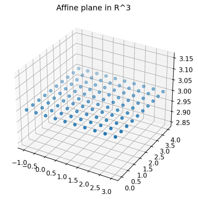
Algebraic difference

A subspace must satisfy closure under addition and scalar multiplication, and must include 0.
An affine subspace is just a subspace plus a fixed shift vector.

Try It Yourself

Define a line in \(\mathbb{R}^2\):

\[
(x,y) = (2,3) + t(1,-1)
\]

Plot it and compare with the subspace spanned by \((1,-1)\).
Construct an affine plane in \(\mathbb{R}^3\) shifted by vector \((5,5,5)\).
Show algebraically that subtracting the shift point turns an affine subspace back into a regular subspace.

The Takeaway

Subspaces go through the origin.
Affine subspaces are shifted copies of subspaces.
They’re essential in geometry, computer graphics, and optimization (e.g., feasible regions in linear programming).

Chapter 5. Linear Transformation and Structure

41. Linear Transformations (Preserving Lines and Sums)

A linear transformation is a function between vector spaces that preserves two key properties:

Additivity: \(T(u+v) = T(u) + T(v)\)
Homogeneity: \(T(cu) = cT(u)\)

In practice, every linear transformation can be represented by a matrix. This lab will help you understand and experiment with linear transformations in Python.

Set Up Your Lab

import numpy as np
import matplotlib.pyplot as plt

Step-by-Step Code Walkthrough

Simple linear transformation (scaling)

Let’s scale vectors by 2 in the x-direction and by 0.5 in the y-direction.

= np.array([
2, 0],
0, 0.5]


= np.array([1, 2])
= A @ v
print("Original v:", v)
print("Transformed Tv:", Tv)

Original v: [1 2]
Transformed Tv: [2. 1.]

Visualizing multiple vectors

= [np.array([1,1]), np.array([2,0]), np.array([-1,2])]

for v in vectors:
= A @ v
0,0,v[0],v[1],head_width=0.1,color='blue',length_includes_head=True)
0,0,Tv[0],Tv[1],head_width=0.1,color='red',length_includes_head=True)

0,color='black',linewidth=0.5)
0,color='black',linewidth=0.5)
-3,5)
-1,5)

"Blue = original, Red = transformed")

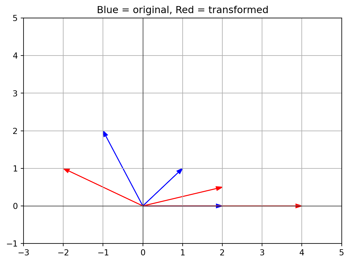
Blue arrows are the original vectors; red arrows are the transformed ones. Notice how the transformation stretches and compresses consistently.

Rotation as a linear transformation

Rotating vectors by \(\theta = 90^\circ\):

= np.pi/2
= np.array([
-np.sin(theta)],



= np.array([1,0])
print("Rotate [1,0] by 90°:", R @ v)

Rotate [1,0] by 90°: [6.123234e-17 1.000000e+00]

The result is \([0,1]\), a perfect rotation.

Checking linearity

= np.array([1,2])
= np.array([3,4])
= 5

= A @ (u+v)
= A@u + A@v
print("Additivity holds?", np.allclose(lhs,rhs))

= A @ (c*u)
= c*(A@u)
print("Homogeneity holds?", np.allclose(lhs,rhs))

Additivity holds? True
Homogeneity holds? True

Both checks return True, proving \(T\) is linear.

Non-linear example (for contrast)

A transformation like \(T(x,y) = (x^2, y)\) is not linear.

def nonlinear(v):
return np.array([v[0]**2, v[1]])

print("T([2,3]) =", nonlinear(np.array([2,3])))

Source link

DZdano

Administrator

Visit Website View All Posts

Step-by-Step Code Walkthrough

Step-by-Step Code Walkthrough

Step-by-Step Code Walkthrough

Step-by-Step Code Walkthrough

Step-by-Step Code Walkthrough

Step-by-Step Code Walkthrough

Step-by-Step Code Walkthrough

Step-by-Step Code Walkthrough

Step-by-Step Code Walkthrough

Step-by-Step Code Walkthrough

Step-by-Step Code Walkthrough

Step-by-Step Code Walkthrough

Step-by-Step Code Walkthrough

Step-by-Step Code Walkthrough

Step-by-Step Code Walkthrough

Step-by-Step Code Walkthrough

Step-by-Step Code Walkthrough

Step-by-Step Code Walkthrough

Step-by-Step Code Walkthrough

Step-by-Step Code Walkthrough

Step-by-Step Code Walkthrough

Step-by-Step Code Walkthrough

Step-by-Step Code Walkthrough

Step-by-Step Code Walkthrough

Step-by-Step Code Walkthrough

Step-by-Step Code Walkthrough

Step-by-Step Code Walkthrough

Step-by-Step Code Walkthrough

Step-by-Step Code Walkthrough

Leave a Reply Cancel reply

Related Stories

Knicks vs. Cavaliers score, live updates, how to watch: Jalen Brunson, James Harden tip off in Game 1 of Eastern Conference finals – Yahoo Sports

What AMD’s Earnings Beat Could Mean for Intel

AMD stock rises on Q1 earnings beat, better-than-expected outlook – Yahoo Finance

You may have missed

Space Horror That Falls Flat

Ubisoft Says New Assassin’s Creed, Far Cry, Ghost Recon Coming…Eventually

Quantic Dream Promises Star Wars Eclipse Is Fine As MOBA Flops

Damon Lindelof Reveals His Canned New Jedi Order Star Wars Film